Linear color interpolation function with adjustable range, baseline, and floor

Usage

col_linear_xf(
  x = 1,
  floor = 0,
  baseline = 0,
  lens = 0,
  n = 6,
  colramp = "Purples",
  open_floor = FALSE,
  floor_color = NULL,
  debug = FALSE,
  ...
)

Arguments

x

numeric value used as a threshold, where numeric values at or above this value x are assigned the last color in the color gradient. Negative values at or below this negative value -x are assigned the first color in the color gradient.

floor

numeric optional value where numeric values between -x and x are assigned the middle color in the color gradient. Note that values at exactly x or -x are assigned the next respective color away from the middle color. When floor=0 or floor=NULL no floor is applied, and colors are assigned using a continuous range of numeric values from -x to x with length n.

baseline

numeric value to define the baseline value, used when zero is not the initial value. Note that baseline can be either higher or lower than x, and colors from colramp will be applied starting at baseline through x.

lens

numeric value indicating a color lens applied to the color gradient, passed to jamba::getColorRamp(). Lens values lens > 0 will condense the color gradient, making smaller changes more visually distinct; lens < 0 expands the color gradient, making smaller changes less visually distinct.

n

integer number of colors used for the initial color gradient. This value is forced to be an odd number, so the "middle color" will always be represented as one strict color. Note that when using a floor, the first non-middle color is used for the floor assignment which means a smaller n value will assign a more visibly distinct color than using a larger n. See examples.

colramp

character passed to jamba::getColorRamp() which recognizes one of several forms of input:

character string matching the name of a color ramp from RColorBrewer (see divergent palettes with RColorBrewer::display.brewer.all(type="div")). Note that adding "_r" will reverse the color gradient, so the default "BuRd_r" will create a color gradient with "blue-white-red" - with red for high values consistent with "heat" in "heatmaps" - where heat is red.
character vector of R colors, which define a specific color ramp. This vector will be expanded to n length.

open_floor

logical indicating whether colors below the assigned floor will still receive non-middle color. Setting open_floor=TRUE is the best method to compare the effect of assigning the strict middle-color to values below the floor, versus using gradient colors below the floor, while all remaining numeric-color assignments are held constant.

floor_color

character default NULL, optional fixed color to apply below the floor threshold. Note that this color works best when open_floor=FALSE.

debug

logical indicating whether to produce a plot that shows the resulting color gradient.

...

additional arguments are ignored.

Value

function that takes numeric input and returns a character vector of colors of the same length.

The color function also recognizes arguments:

'return_rgb': logical whether to return R,G,B as a matrix, default FALSE.
'max_value': numeric with maximum RGB values, default 1.

The object contains attributes:

'legend_at': numeric vector of legend label positions.
'legend_labels': character vector of labels associated with the 'legend_at' positions. When floor is used, the labels include positions just below floor, and the label indicates '<floor', for example '<1.5'. The label is used by scale_color_div_xf() for the ggplot2 legend.

Details

This function is the linear equivalent of col_div_xf(), in that it takes linear/sequential color gradient instead of a divergent color gradient.

Examples

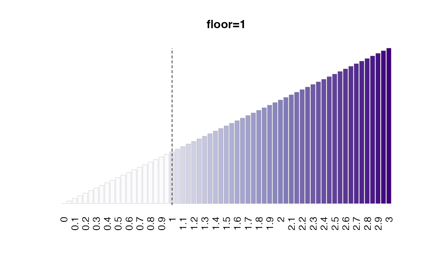
col_fn1 <- col_linear_xf(x=3, baseline=0, floor=0)
col_fn2 <- col_linear_xf(x=3, baseline=0, floor=1)

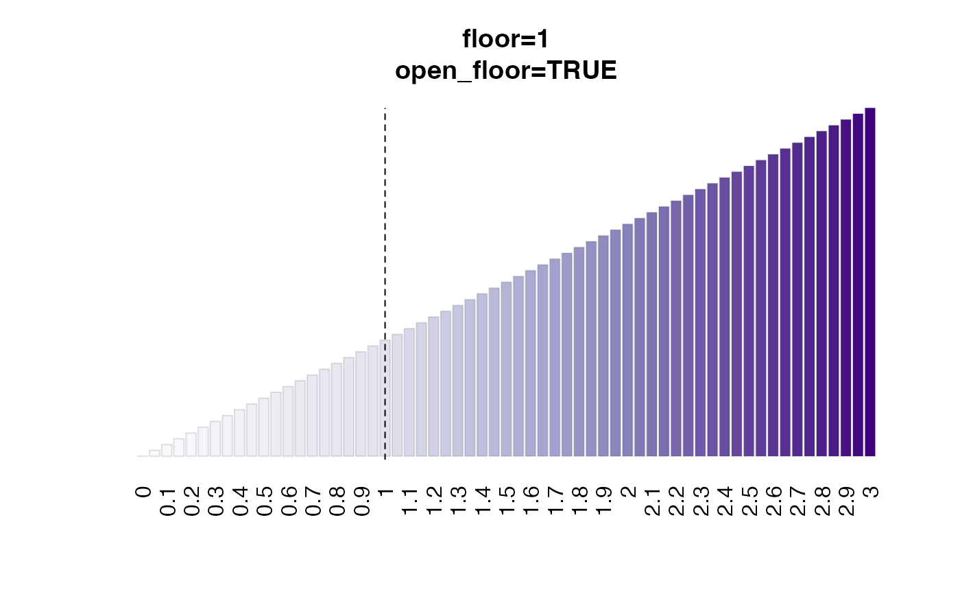
col_fn2o <- col_linear_xf(x=3, baseline=0, floor=1, open_floor=TRUE)

test_seq <- seq(from=0, to=3, by=0.05);
names(test_seq) <- round(test_seq, digits=2);

opar <- par("mfrow"=c(1, 1));
bp0 <- barplot(abs(test_seq),
   las=2, yaxt="n",
   main="floor=0",
   col=col_fn1(test_seq),
   border="#22222222")
abline(v=bp0[abs(test_seq) == 1,], lty="dashed")

bp1 <- barplot(abs(test_seq),
   las=2, yaxt="n",
   main="floor=1",
   col=col_fn2(test_seq),
   border="#22222222")
abline(v=bp1[abs(test_seq) == 1,], lty="dashed")

bp2 <- barplot(abs(test_seq),
   las=2, yaxt="n",
   main="floor=1\nopen_floor=TRUE",
   col=col_fn2o(test_seq),
   border="#22222222")
abline(v=bp2[abs(test_seq) == 1,], lty="dashed")

par(opar)

col_fn3 <- col_linear_xf(x=3, baseline=6, floor=5)
test_seq <- seq(from=0, to=7, by=0.1);
names(test_seq) <- round(test_seq, digits=2);
bp3 <- barplot(abs(test_seq),
   las=2, yaxt="n",
   main="baseline=6, x=3, floor=5",
   col=col_fn3(test_seq),
   border="#22222222")
abline(v=bp3[abs(test_seq) == 5,], lty="dashed")
abline(v=bp3[abs(test_seq) == 3,], lty="dashed")


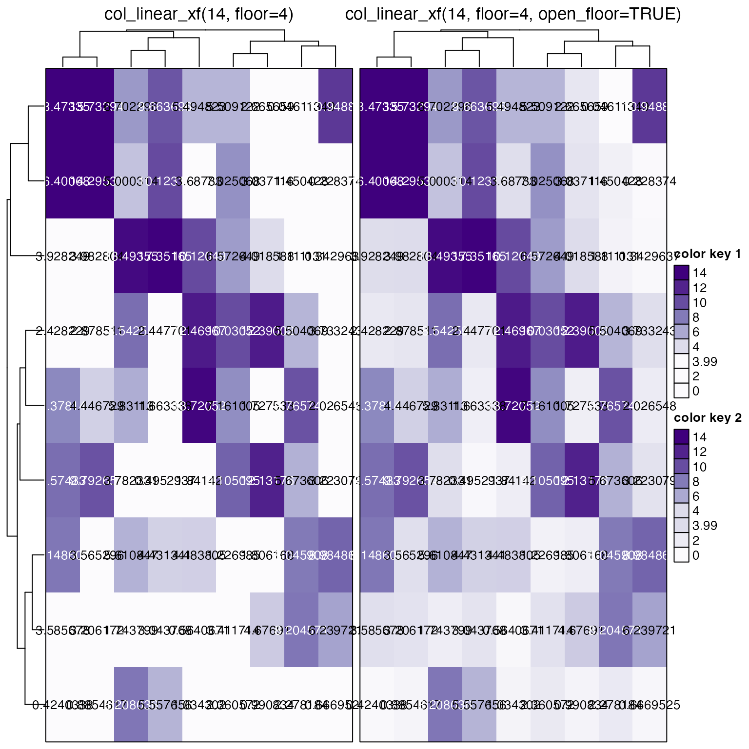
# Optionally show how to display data and legend in ComplexHeatmap
if (jamba::check_pkg_installed("ComplexHeatmap")) {
   set.seed(123);
   m <- abs(matrix(ncol=9, rnorm(81) * 8));
   col1 <- col_linear_xf(14, floor=4, n=8, lens=2);
   hm_1 <- ComplexHeatmap::Heatmap(m, col=col1,
      cell_fun=jamba::cell_fun_label(m=m, col_hm=col1),
      heatmap_legend_param=list(
         color_bar="discrete",
         at=c(0, 2, 3.99, 4, 6, 8, 10, 12, 14),
         border=TRUE),
      column_title="col_linear_xf(14, floor=4)",
      name="color key 1",
      border=TRUE);

   col2 <- col_linear_xf(14, floor=4, n=8, lens=2, open_floor=TRUE);
   hm_2 <- ComplexHeatmap::Heatmap(m,
      col=col2,
      cell_fun=jamba::cell_fun_label(m=m, col_hm=col2),
      heatmap_legend_param=list(
         color_bar="discrete",
         at=c(0, 2, 3.99, 4, 6, 8, 10, 12, 14),
         border=TRUE),
      column_title="col_linear_xf(14, floor=4, open_floor=TRUE)",
      name="color key 2",
      border=TRUE);
   hm_1 + hm_2
}