Compute contrast statistics on SummarizedExperiment data
Source:R/jam_secontrasts.R
se_contrast_stats.RdCompute contrast statistics on SummarizedExperiment data
Usage
se_contrast_stats(
  se,
  assay_names,
  adjp_cutoff = 0.05,
  p_cutoff = NULL,
  fold_cutoff = 1.5,
  int_adjp_cutoff = adjp_cutoff,
  int_p_cutoff = p_cutoff,
  int_fold_cutoff = fold_cutoff,
  mgm_cutoff = NULL,
  ave_cutoff = NULL,
  confint = FALSE,
  floor_min = NULL,
  floor_value = NULL,
  sedesign = NULL,
  icontrasts = NULL,
  idesign = NULL,
  igenes = NULL,
  isamples = NULL,
  enforce_design = TRUE,
  use_voom = FALSE,
  voom_block_twostep = TRUE,
  posthoc_test = c("none", "DEqMS"),
  posthoc_args = list(DEqMS = list(PSM_counts = NULL, fit.method = "loess")),
  weights = NULL,
  robust = FALSE,
  handle_na = c("full1", "full", "partial", "all", "none"),
  na_value = 0,
  rowData_colnames = c("SYMBOL"),
  collapse_by_gene = FALSE,
  block = NULL,
  correlation = NULL,
  max_correlation_rows = 10000,
  normgroup = NULL,
  do_normgroups = TRUE,
  seed = 123,
  verbose = FALSE,
  ...
)
Arguments
- se
SummarizedExperimentobject.Note that
colnames(se)should match the samples insedesign, or therownames(idesign)whensedesignis not supplied.Data is subset by
colnames(se)usingisampleswhen supplied, andrownames(se)whenigenesis supplied.Note argument
rowData_colnamescan be used to retain somerowData(se)columns in the statdata.framesummaries for convenience, particularly helpful when analyzing microarray data where therownames(se)represent probe ID or assay ID.
- assay_names
charactervector with one or more assay names fromnames(assays(se)).- adjp_cutoff
numericvalue threshold with the adjusted P-value at or below which a contrast result can be considered a statistical hit. This threshold is applied in addition to othercutoffvalues.- p_cutoff
numericvalue threshold with the unadjusted P-value at or below which a contrast result can be considered a statistical hit. This argument is not recommended, in favor of usingadjp_cutoff. This threshold is applied in addition to othercutoffvalues.- fold_cutoff
numericvalue threshold indicating the normal absolute fold change at or above which a contrast result can be considered a statistical hit. For clarity, this threshold is normal space fold change, for example 2-fold would befold_cutoff=2.- int_adjp_cutoff, int_p_cutoff, int_fold_cutoff
optional thresholds used only when a two-way interaction style contrast is detected. These optional thresholds may be useful to apply more lenient criteria to interaction contrasts, but in that event are cautioned to be used for data mining exercises. Ideally, the thresholds are identical between pairwise and interaction contrasts, and ideally there are enough replicates in the data to support the interaction contrasts with sufficient confidence to make those comparisons.
- mgm_cutoff
numericvalue threshold of the maximum group mean value required in each contrast for the contrast to be considered a statistical hit. The "max group mean" logic requires only one group in a contrast to be above this threshold, while all other groups can have values below the threshold. This threshold is applied in addition to othercutoffvalues.- ave_cutoff
numericvalue threshold of the average expression as reported bylimma::lmFit(), within each normgroup if relevant, for the contrast to be considered a statistical hit. This threshold is applied in addition to othercutoffvalues. Typically the column "AvgExpr" is calculated as a row mean.- confint
logicalpassed tolimma::topTable()indicating whether to calculate 95% confidence intervals for log2 fold changelogFCvalues. Alternatively it can be anumericvalue between zero and one specifying a specific confidence interval.- floor_min, floor_value
numericminimum value (floor_min) at or below whichnumericvalues in the assay data matrix are reverted tofloor_valueas a replacement. This option is valuable to set allnumericvalues at or below zero to zero, or to set all values at or below zero toNAin circumstances where zero indicates "no measurement" and would be more accurately represented as a missing measurement than a measurement of0.Note:
floor_minis applied beforehandle_na, so that this step is able to createNAvalues which will be handled appropriately based upon the optionhandle_na.
- sedesign
SEDesignobject as defined bygroups_to_sedesign(), with slotNames"design","contrasts", and"samples". The argumentsidesignandicontrastsare ignored when this argument is defined.- icontrasts, idesign
numericmatrices representing statistical contrasts, and sample-group design matrices. These values are ignored whensedesignis defined.- igenes
charactervector with optional subset ofrownames(se), by default it uses allrownames(se).- isamples
charactervector with optional subset ofcolnames(se), by default it usescolnames(se)that are also defined in the design matrix.- enforce_design
logical(this option is not implemented). By default the design matrix is used to subset the inputcolnames(se)as needed, andisamplesis used to subset the design matrix and corresponding contrasts as relevant.- use_voom
logicalindicating whether to applylimma-voomanalysis steps. When applied, data is not scaled usinglimma:voom(), instead uses data as supplied.- voom_block_twostep
logicalindicating whether to perform the "two-step" voom methodology whenblockis also supplied. This workflow is recommended by voom authors:call
voom()first withoutblockto determine overallweightscall
duplicateCorrelation()if necessary, using the voomweights, and theblockargument, to calculatecorrelation.call
voom()again using thecorrelation,weights, andblockarguments. This produces improvedweights.call
duplicateCorrelation()again with the updatedweights, andblockin order to calculate improvedcorrelation.Then proceed with
lmFit()using appropriateweightsusingblock; and appropriatecorrelationalso using the properweightsandblock.
- posthoc_test
characterstring indicating an optional post-hoc test to apply."none": applieslimma::eBayes()by default, the moderated t-test."DEqMS": applies adjustment for proteomics measurements provided by the package"DEqMS". Seeposthoc_args.
- posthoc_args
listnamed by theposthoc_testabove."DEqMS"recognizes two arguments, which are passed toDEqMS::spectraCounteBayes():"PSM_counts": anumericvector of peptide spectra matched, one perigenesorrownames(se). These values are used by DEqMS to model variability based upon the number of spectra as the key measure of confidence."fit.method":charactername of the model to use, default is"loess".
- weights
numericnon-negative precision weights passed tolimma::lmFit(), either as a matrix with nrow and ncol that matchigenesandisamples, respectively, or matching one oflength(igenes)orlength(isamples). Whenigenesorisamplesare not supplied, it usesnrow(se)orncol(se), respectively.- robust
logicalpassed tolimma::eBayes(), whether estimation ofdf.priorandvar.priorshould be robust against outlier sample variances.- handle_na
characterstring indicating how to handleNAvalues in the data matrix, passed tohandle_na_values()."partial": ReplaceNAvalues withna_value, except when an entire group isNAthe entire group is kept atNA."full": RetainNAvalues, except when an entire group isNAthe replicate values are replaced withna_value. The option"full1"may be preferred, since it only replaces one value in the group, therefore does not misrepresent the variability of the group as zero."full1": RetainNAvalues, except when an entire group isNA, one replicate value in the group is replaced withna_value. By replacing only one replicate withna_valuethe group does not have a variance/dispersion, forcing the variance to be determined by the other group in the contrast, while still allowing an approximate fold change to be calculated. This option is suitable when there is a noise floor above zero, as it retains an approximate fold change while estimating a P-value using only the variance derived from the non-NAgroup."all": replace allNAvalues withna_value."none": perform no replacement ofNAvalues.
- na_value
numericpassed tohandle_na_values()- rowData_colnames
charactervector of colnames inrowData(se)that should be retained in each statdata.frameproduced as output. The values inrowData_colnamesare intersected withcolnames(rowData(se))to determine which columns to keep.- collapse_by_gene
logical(not currently implemented).- block
character,factor, ornumericused as a blocking factor, using argumentblockinlimma::lmFit()for example.The argument can be supplied as one of the following:
characterwith one or morecolnames(colData(se))charactervector named using values inisamplesand/orcolnames(se)charactervector without names, whose length must equallength(isamples)or whenisamplesis not provided,ncol(se).
- correlation
optional inter-duplicate or inter-technical correlation matrix passed to
limma::lmFit().- max_correlation_rows
numericmaximum number of rows inimatrixto use when callinglimma::duplicateCorrelation(). This process only occurs whenblockis defined,correlation=NULLandnrow(imatrix) > max_correlation_rows. In this scenario, a random subset of rows are used to calculatecorrelation, then thatcorrelationis used forlimma::lmFit(). This process is intended to help very large data volumes, where the speed oflimma::duplicateCorrelation()is impacted in quadratic manner by increasing number of rows, while also not improving the summary correlation value.- normgroup
characterorfactorvector with lengthncol(se)orlength(isamples)whenisamplesis defined. Values define independent normalization groups, which performs independent analyses within each unique normalization group. This option is intended for convenience, enabling separate variance models for each normalization group, which is appropriate when analyzing very different sample types. During limma model fit, all samples in all groups are used by default, which may incorrectly estimate variance when the variability by row is not uniform across different sample types. Whennormgroup=NULLthe default is to assume all samples are in the samenormgroup="bulk". Each subset of samples begins with the samesedesign,idesign,icontrast, however they are fed intovalidate_sestats()to subset the appropriate contrasts to use only samples within the current normgroup. As a result, any contrasts that span two normgroups will be removed, and will not appear in the output.The argument can be supplied as one of the following:
characterwith one or morecolnames(colData(se))charactervector named using values inisamplesand/orcolnames(se)charactervector without names, whose length must equallength(isamples)or whenisamplesis not provided,ncol(se).
- do_normgroups
logicalwhether to enable normgroup processing, or to use the previous technique that kept all samples together. This argument may be removed in future, with recommendation to usenormgroup=NULLto disable normalization group processing. Note that whennormgroup=NULLthe output should be identical withdo_normgroups=TRUEanddo_normgroups=FALSE.- seed
numericused to set a random seed withset.seed()for reproducibility. Useseed=NULLto avoid setting a random seed. Note this action will only affect downstream functions that employ some form of randomization.- verbose
logicalindicating whether to print verbose output.- ...
additional arguments are ignored.
Details
This function is essentially a wrapper around statistical methods
in the limma package, with additional steps to apply statistical
thresholds to define "statistical hits" by three main criteria:
P-value or adjusted P-value
fold change
max group mean
This function is unique in that it applies the statistical methods
to one or more "signals" in the input SummarizedExperiment assays,
specifically intended to compare things like normalization methods.
If multiple statistical thresholds are defined, each one is applied in order, which is specifically designed to compare the effect of applying different statistical thresholds. For example one may want to pre-compute "statistical hits" using adjusted P-value 0.05, and 0.01; or using fold change >= 1.5, or fold change >= 2.0. The underlying statistics are the same, but a column indicating hits is created for each set of thresholds.
Hits are annotated:
-1for down-regulation0for un-changed (by the given criteria)1for up-regulation
The results are therefore intended to feed directional Venn diagrams, which display the overlapping gene hits, and whether the directions are shared or opposed.
This function can optionally apply the limma-voom workflow,
which involves calculating matrix weights using limma::voom(),
then applying those weights during the model fit.
The output is intended to include several convenient formats:
stats_dfs- list ofdata.framestats one per contraststats_df- onedata.framewith all stats togetherhit_array-arraywith three dimensions: signal; contrast; threshold whose cells contain hit flags (-1, 0, 1) named byrownames(se).
Design and contrast matrices can be defined using the function
jamses::groups_to_sedesign(). That function assigns each sample
to a sample group, then assembles all relevant group contrasts
which involve only one-factor contrast at a time. It optionally
defines two-factor contrasts (contrast of contrasts) where
applicable.
A subset of genes (rownames(se)) or samples (colnames(se)) can
be defined, to restrict calculations to use only the subset data.
See also
Other jamses stats:
ebayes2dfs(),
format_hits(),
handle_na_values(),
hit_array_to_list(),
process_sestats_to_hitim(),
run_limma_replicate(),
save_sestats(),
sestats_to_dfs(),
sestats_to_df(),
voom_jam()
Examples
set.seed(123)
expr <- rnorm(20) + 7;
noise <- rnorm(120) / 5;
fold <- rnorm(20) / 2.5;
m <- matrix(expr + noise, ncol=6);
for (i in 4:6) {
m[,i] <- m[,i] + fold;
}
# m <- matrix(rnorm(120)/2 + 5, ncol=6);
colnames(m) <- paste0(rep(c("Vehicle", "Treated"), each=3), 1:3)
rownames(m) <- paste0("row", seq_len(20))
# simulate some "hits"
m[1, 4:6] <- m[1, 4:6] + 2
m[2, 4:6] <- m[2, 4:6] + 1.5
m[3, 4:6] <- m[3, 4:6] - 1.3
# create SummarizedExperiment
se <- SummarizedExperiment::SummarizedExperiment(
assays=list(counts=m),
colData=data.frame(sample=colnames(m),
group=factor(rep(c("Vehicle", "Treated"), each=3),
c("Vehicle", "Treated"))),
rowData=data.frame(measurement=rownames(m)))
# assign colors
sample_color_list <- platjam::design2colors(se)
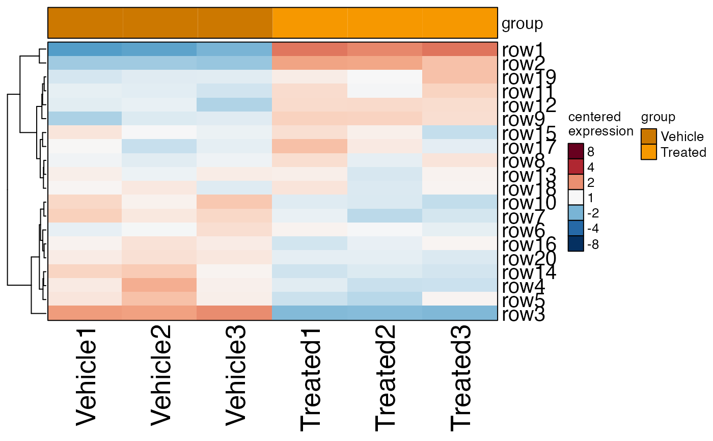
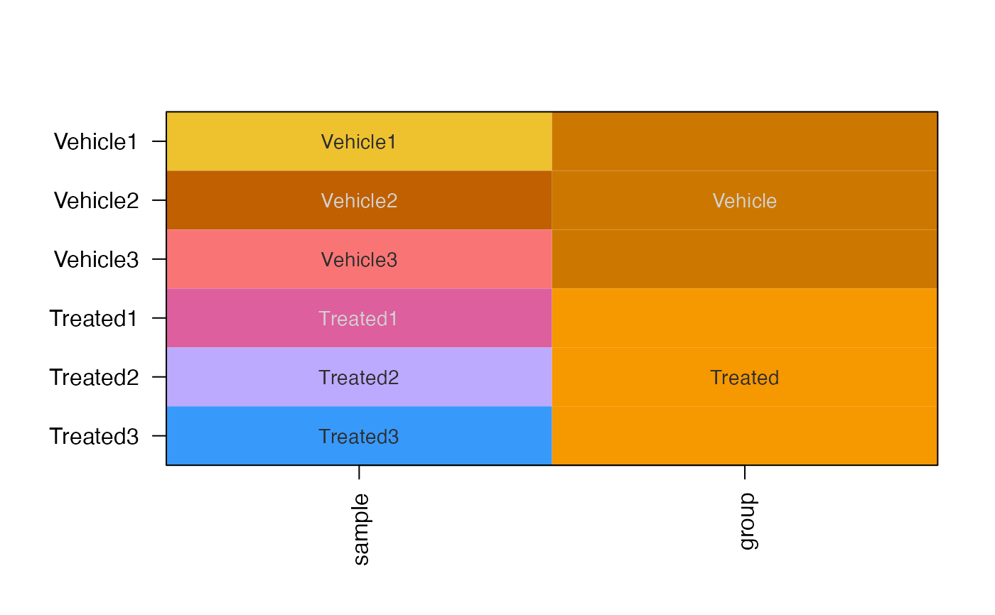 # heatmap
heatmap_se(se, sample_color_list=sample_color_list)
# heatmap
heatmap_se(se, sample_color_list=sample_color_list)
 # create SEDesign
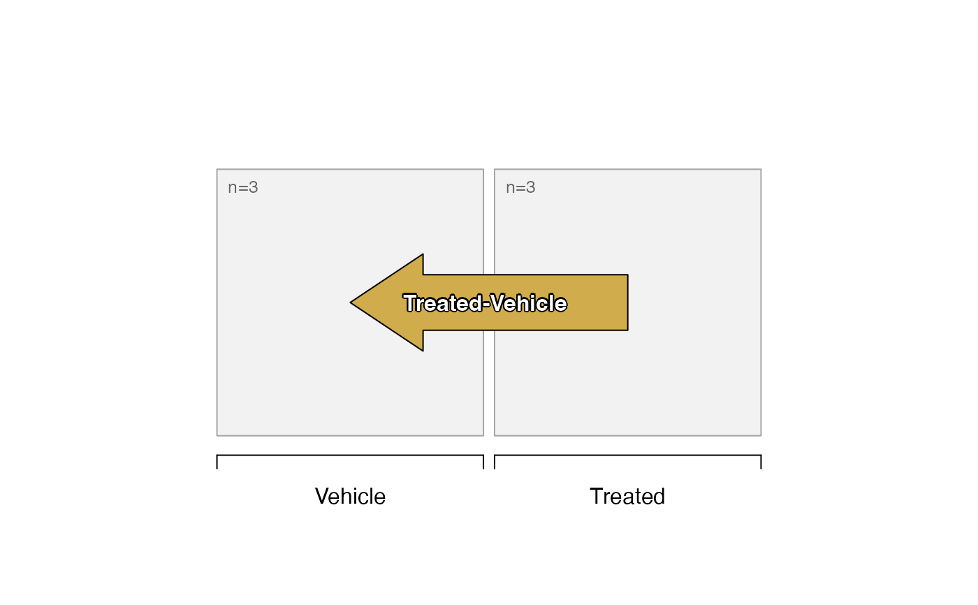
sedesign <- groups_to_sedesign(se, group_colnames="group")
# plot the design and contrasts
plot_sedesign(sedesign)
#> Warning: no non-missing arguments to max; returning -Inf
#> Warning: no non-missing arguments to max; returning -Inf
# create SEDesign
sedesign <- groups_to_sedesign(se, group_colnames="group")
# plot the design and contrasts
plot_sedesign(sedesign)
#> Warning: no non-missing arguments to max; returning -Inf
#> Warning: no non-missing arguments to max; returning -Inf
 # limma contrasts
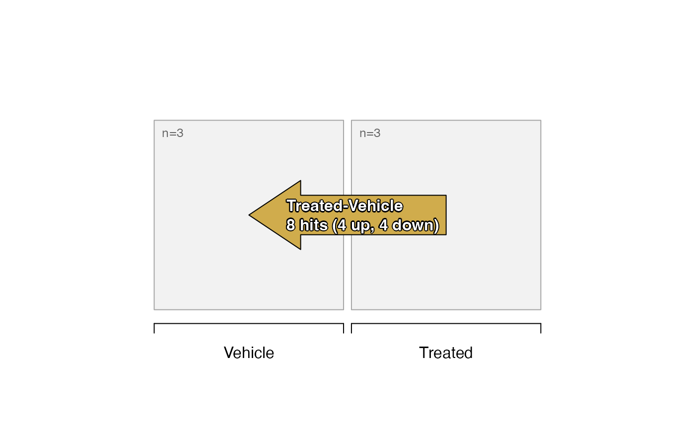
sestats <- se_contrast_stats(se=se,
sedesign=sedesign,
assay_names="counts")
# print data.frame summary of hits
sestats_to_df(sestats)
#> Signal Contrasts hit adjp0.05 fc1.5
#> Treated-Vehicle counts Treated-Vehicle 8 hits (4 up, 4 down)
# plot the design with number of hits labeled
plot_sedesign(sedesign, sestats=sestats)
#> Warning: no non-missing arguments to max; returning -Inf
#> Warning: no non-missing arguments to max; returning -Inf
# limma contrasts
sestats <- se_contrast_stats(se=se,
sedesign=sedesign,
assay_names="counts")
# print data.frame summary of hits
sestats_to_df(sestats)
#> Signal Contrasts hit adjp0.05 fc1.5
#> Treated-Vehicle counts Treated-Vehicle 8 hits (4 up, 4 down)
# plot the design with number of hits labeled
plot_sedesign(sedesign, sestats=sestats)
#> Warning: no non-missing arguments to max; returning -Inf
#> Warning: no non-missing arguments to max; returning -Inf
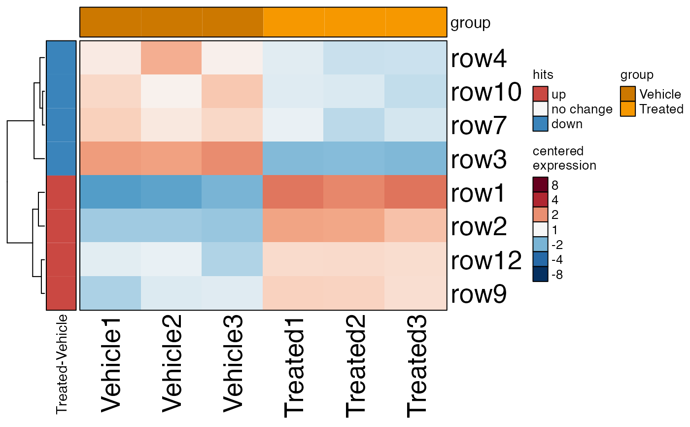
 # heatmap with hits
heatmap_se(se,
sample_color_list=sample_color_list,
sestats=sestats)
# heatmap with hits
heatmap_se(se,
sample_color_list=sample_color_list,
sestats=sestats)
 # review stats table
stats_df <- sestats$stats_dfs$counts[["Treated-Vehicle"]]
head(stats_df)
#> probes hit adjp0.05 fc1.5 Treated-Vehicle logFC Treated-Vehicle
#> row1 row1 1 2.3337734
#> row2 row2 1 1.4366480
#> row3 row3 -1 -1.8277444
#> row4 row4 -1 -0.6312502
#> row5 row5 0 -0.5632394
#> row6 row6 0 -0.0696241
#> fold Treated-Vehicle P.Value Treated-Vehicle adj.P.Val Treated-Vehicle
#> row1 5.041222 6.410602e-17 1.282120e-15
#> row2 2.706912 2.127696e-11 1.418464e-10
#> row3 -3.549816 3.099395e-14 3.099395e-13
#> row4 -1.548907 3.752311e-04 9.143257e-04
#> row5 -1.477583 1.285519e-03 2.571038e-03
#> row6 -1.049443 6.392157e-01 7.102397e-01
#> mgm Treated-Vehicle Vehicle mean Treated mean
#> row1 8.681105 6.347332 8.681105
#> row2 8.144589 6.707941 8.144589
#> row3 8.383734 8.383734 6.555990
#> row4 7.098608 7.098608 6.467357
#> row5 7.096697 7.096697 6.533457
#> row6 8.547980 8.547980 8.478356
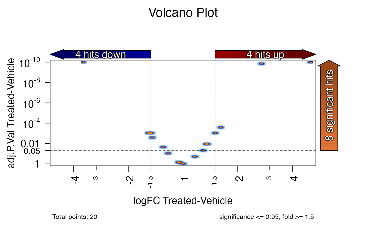
# volcano plot for one contrast
jamma::volcano_plot(stats_df)
#> ## (14:56:43) 28Oct2024: volcano_plot(): sig_colname: adj.P.Val Treated-Vehicle
#> ## (14:56:43) 28Oct2024: volcano_plot(): lfc_colname: logFC Treated-Vehicle
# review stats table
stats_df <- sestats$stats_dfs$counts[["Treated-Vehicle"]]
head(stats_df)
#> probes hit adjp0.05 fc1.5 Treated-Vehicle logFC Treated-Vehicle
#> row1 row1 1 2.3337734
#> row2 row2 1 1.4366480
#> row3 row3 -1 -1.8277444
#> row4 row4 -1 -0.6312502
#> row5 row5 0 -0.5632394
#> row6 row6 0 -0.0696241
#> fold Treated-Vehicle P.Value Treated-Vehicle adj.P.Val Treated-Vehicle
#> row1 5.041222 6.410602e-17 1.282120e-15
#> row2 2.706912 2.127696e-11 1.418464e-10
#> row3 -3.549816 3.099395e-14 3.099395e-13
#> row4 -1.548907 3.752311e-04 9.143257e-04
#> row5 -1.477583 1.285519e-03 2.571038e-03
#> row6 -1.049443 6.392157e-01 7.102397e-01
#> mgm Treated-Vehicle Vehicle mean Treated mean
#> row1 8.681105 6.347332 8.681105
#> row2 8.144589 6.707941 8.144589
#> row3 8.383734 8.383734 6.555990
#> row4 7.098608 7.098608 6.467357
#> row5 7.096697 7.096697 6.533457
#> row6 8.547980 8.547980 8.478356
# volcano plot for one contrast
jamma::volcano_plot(stats_df)
#> ## (14:56:43) 28Oct2024: volcano_plot(): sig_colname: adj.P.Val Treated-Vehicle
#> ## (14:56:43) 28Oct2024: volcano_plot(): lfc_colname: logFC Treated-Vehicle
 ###############################
# simulate a two-way model
adjust <- rnorm(20);
new_fold <- rnorm(20);
se2 <- cbind(se, se)
groups2 <- paste0(rep(c("WT", "KO"), each=6),
"_",
SummarizedExperiment::colData(se)$group)
groups2 <- factor(groups2, levels=unique(groups2))
colnames(se2) <- paste0(groups2, 1:3)
SummarizedExperiment::colData(se2)$sample <- colnames(se2);
SummarizedExperiment::colData(se2)$group <- groups2;
SummarizedExperiment::colData(se2)$genotype <- jamba::gsubOrdered("_.+", "",
SummarizedExperiment::colData(se2)$group)
SummarizedExperiment::colData(se2)$treatment <- jamba::gsubOrdered("^.+_", "",
SummarizedExperiment::colData(se2)$group)
SummarizedExperiment::assays(se2)$counts[,7:12] <- (
SummarizedExperiment::assays(se2)$counts[,7:12] + adjust)
SummarizedExperiment::assays(se2)$counts[,10:12] <- (
SummarizedExperiment::assays(se2)$counts[,10:12] + new_fold)
# assign colors
sample_color_list2 <- platjam::design2colors(se2,
class_colnames="genotype",
color_sub=c(
Vehicle="palegoldenrod",
Treated="firebrick4"),
group_colnames="group")
###############################
# simulate a two-way model
adjust <- rnorm(20);
new_fold <- rnorm(20);
se2 <- cbind(se, se)
groups2 <- paste0(rep(c("WT", "KO"), each=6),
"_",
SummarizedExperiment::colData(se)$group)
groups2 <- factor(groups2, levels=unique(groups2))
colnames(se2) <- paste0(groups2, 1:3)
SummarizedExperiment::colData(se2)$sample <- colnames(se2);
SummarizedExperiment::colData(se2)$group <- groups2;
SummarizedExperiment::colData(se2)$genotype <- jamba::gsubOrdered("_.+", "",
SummarizedExperiment::colData(se2)$group)
SummarizedExperiment::colData(se2)$treatment <- jamba::gsubOrdered("^.+_", "",
SummarizedExperiment::colData(se2)$group)
SummarizedExperiment::assays(se2)$counts[,7:12] <- (
SummarizedExperiment::assays(se2)$counts[,7:12] + adjust)
SummarizedExperiment::assays(se2)$counts[,10:12] <- (
SummarizedExperiment::assays(se2)$counts[,10:12] + new_fold)
# assign colors
sample_color_list2 <- platjam::design2colors(se2,
class_colnames="genotype",
color_sub=c(
Vehicle="palegoldenrod",
Treated="firebrick4"),
group_colnames="group")
 # heatmap
hm2a <- heatmap_se(se2,
sample_color_list=sample_color_list2,
controlSamples=1:3,
center_label="versus WT_Vehicle",
column_title_rot=60,
row_cex=0.4,
column_cex=0.5,
column_title_gp=grid::gpar(fontsize=8),
column_split="group")
ComplexHeatmap::draw(hm2a, column_title=attr(hm2a, "hm_title"), merge_legends=TRUE)
# heatmap
hm2a <- heatmap_se(se2,
sample_color_list=sample_color_list2,
controlSamples=1:3,
center_label="versus WT_Vehicle",
column_title_rot=60,
row_cex=0.4,
column_cex=0.5,
column_title_gp=grid::gpar(fontsize=8),
column_split="group")
ComplexHeatmap::draw(hm2a, column_title=attr(hm2a, "hm_title"), merge_legends=TRUE)
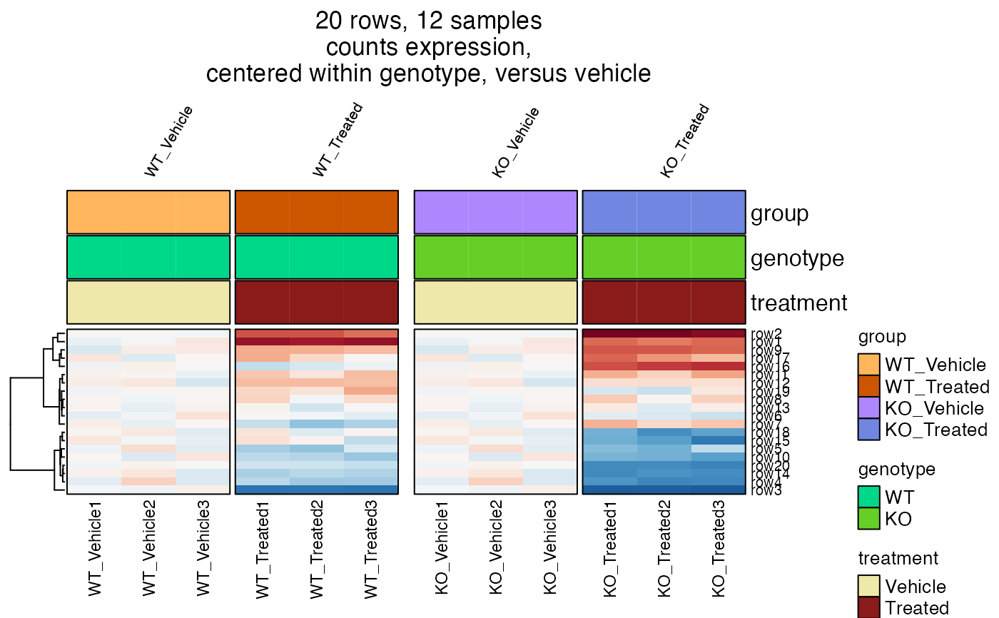
 # heatmap centered by genotype
hm2b <- heatmap_se(se2,
sample_color_list=sample_color_list2,
controlSamples=c(1:3, 7:9),
control_label="versus vehicle",
column_gap=grid::unit(c(1, 3, 1), "mm"),
centerby_colnames="genotype",
column_title_rot=60,
row_cex=0.4,
column_cex=0.5,
column_title_gp=grid::gpar(fontsize=8),
column_split="group")
ComplexHeatmap::draw(hm2b, column_title=attr(hm2b, "hm_title"), merge_legends=TRUE)
# heatmap centered by genotype
hm2b <- heatmap_se(se2,
sample_color_list=sample_color_list2,
controlSamples=c(1:3, 7:9),
control_label="versus vehicle",
column_gap=grid::unit(c(1, 3, 1), "mm"),
centerby_colnames="genotype",
column_title_rot=60,
row_cex=0.4,
column_cex=0.5,
column_title_gp=grid::gpar(fontsize=8),
column_split="group")
ComplexHeatmap::draw(hm2b, column_title=attr(hm2b, "hm_title"), merge_legends=TRUE)
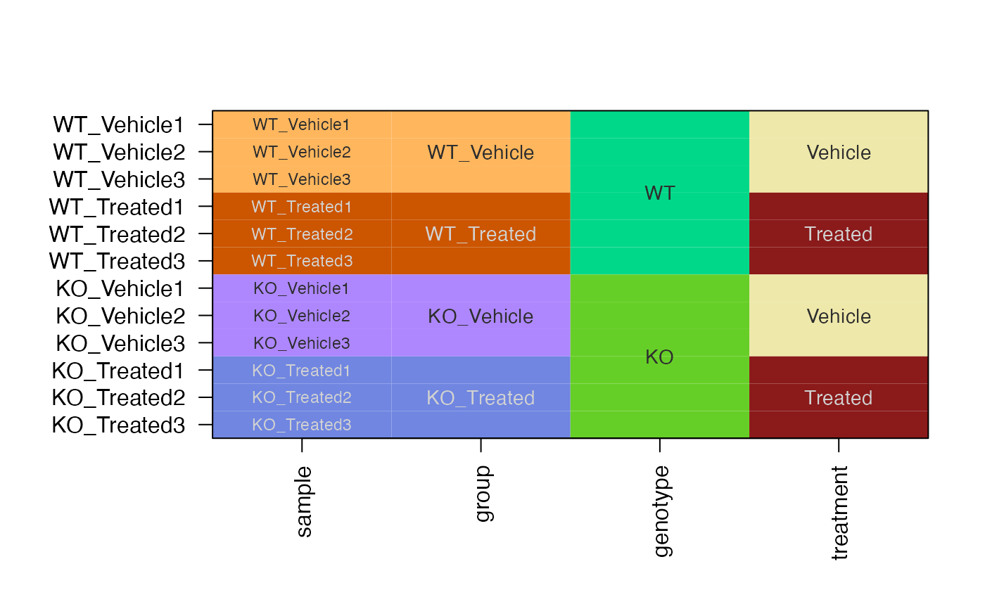
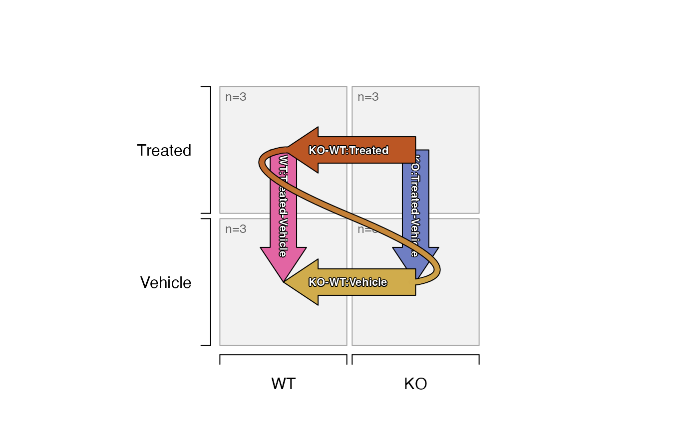
 # create SEDesign
sedesign2 <- groups_to_sedesign(se2, group_colnames="group")
# plot the design and contrasts
plot_sedesign(sedesign2, label_cex=0.7)
# create SEDesign
sedesign2 <- groups_to_sedesign(se2, group_colnames="group")
# plot the design and contrasts
plot_sedesign(sedesign2, label_cex=0.7)
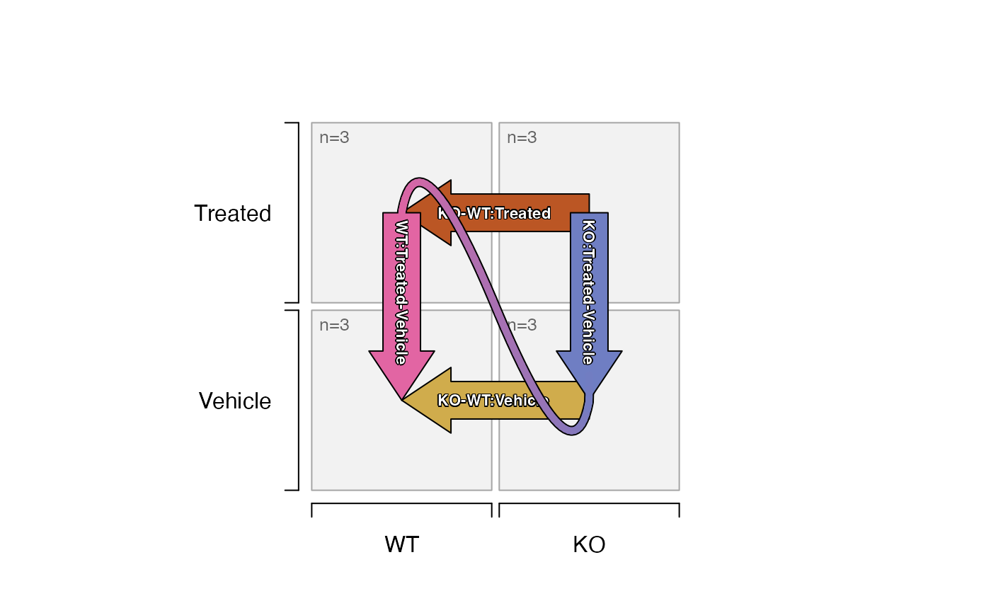
 # note the two-way contrast can be flipped
plot_sedesign(sedesign2, flip_twoway=TRUE, label_cex=0.7)
# note the two-way contrast can be flipped
plot_sedesign(sedesign2, flip_twoway=TRUE, label_cex=0.7)
 # limma contrasts
sestats2 <- se_contrast_stats(se=se2,
sedesign=sedesign2,
assay_names="counts")
# print data.frame summary of hits
sestats_to_df(sestats2)
#> Signal
#> KO_Vehicle-WT_Vehicle counts
#> KO_Treated-WT_Treated counts
#> WT_Treated-WT_Vehicle counts
#> KO_Treated-KO_Vehicle counts
#> (KO_Treated-WT_Treated)-(KO_Vehicle-WT_Vehicle) counts
#> Contrasts
#> KO_Vehicle-WT_Vehicle KO_Vehicle-WT_Vehicle
#> KO_Treated-WT_Treated KO_Treated-WT_Treated
#> WT_Treated-WT_Vehicle WT_Treated-WT_Vehicle
#> KO_Treated-KO_Vehicle KO_Treated-KO_Vehicle
#> (KO_Treated-WT_Treated)-(KO_Vehicle-WT_Vehicle) (KO_Treated-WT_Treated)-(KO_Vehicle-WT_Vehicle)
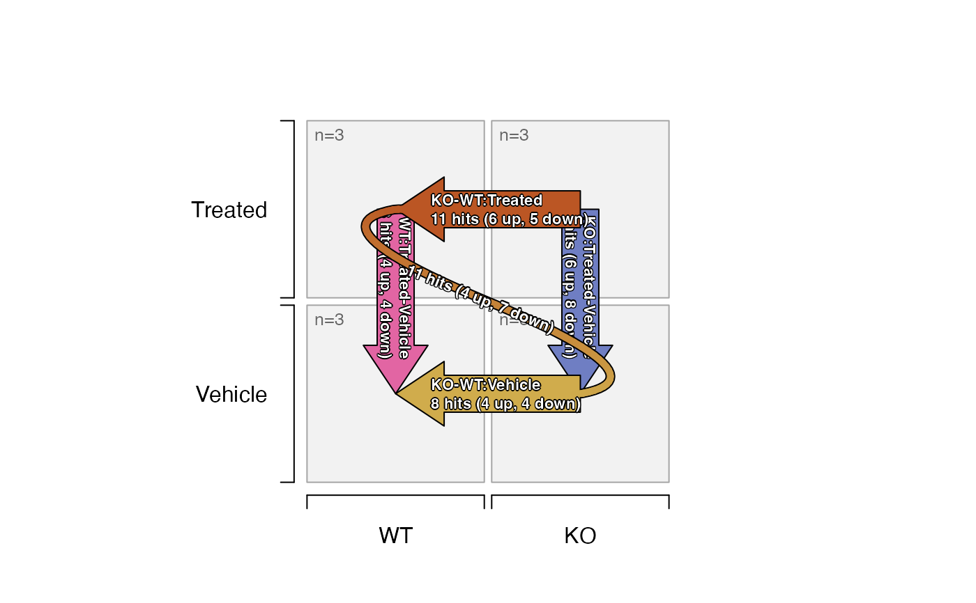
#> hit adjp0.05 fc1.5
#> KO_Vehicle-WT_Vehicle 8 hits (4 up, 4 down)
#> KO_Treated-WT_Treated 11 hits (6 up, 5 down)
#> WT_Treated-WT_Vehicle 8 hits (4 up, 4 down)
#> KO_Treated-KO_Vehicle 14 hits (6 up, 8 down)
#> (KO_Treated-WT_Treated)-(KO_Vehicle-WT_Vehicle) 11 hits (4 up, 7 down)
# plot the design with number of hits labeled
plot_sedesign(sedesign2, sestats=sestats2, label_cex=0.7)
# limma contrasts
sestats2 <- se_contrast_stats(se=se2,
sedesign=sedesign2,
assay_names="counts")
# print data.frame summary of hits
sestats_to_df(sestats2)
#> Signal
#> KO_Vehicle-WT_Vehicle counts
#> KO_Treated-WT_Treated counts
#> WT_Treated-WT_Vehicle counts
#> KO_Treated-KO_Vehicle counts
#> (KO_Treated-WT_Treated)-(KO_Vehicle-WT_Vehicle) counts
#> Contrasts
#> KO_Vehicle-WT_Vehicle KO_Vehicle-WT_Vehicle
#> KO_Treated-WT_Treated KO_Treated-WT_Treated
#> WT_Treated-WT_Vehicle WT_Treated-WT_Vehicle
#> KO_Treated-KO_Vehicle KO_Treated-KO_Vehicle
#> (KO_Treated-WT_Treated)-(KO_Vehicle-WT_Vehicle) (KO_Treated-WT_Treated)-(KO_Vehicle-WT_Vehicle)
#> hit adjp0.05 fc1.5
#> KO_Vehicle-WT_Vehicle 8 hits (4 up, 4 down)
#> KO_Treated-WT_Treated 11 hits (6 up, 5 down)
#> WT_Treated-WT_Vehicle 8 hits (4 up, 4 down)
#> KO_Treated-KO_Vehicle 14 hits (6 up, 8 down)
#> (KO_Treated-WT_Treated)-(KO_Vehicle-WT_Vehicle) 11 hits (4 up, 7 down)
# plot the design with number of hits labeled
plot_sedesign(sedesign2, sestats=sestats2, label_cex=0.7)
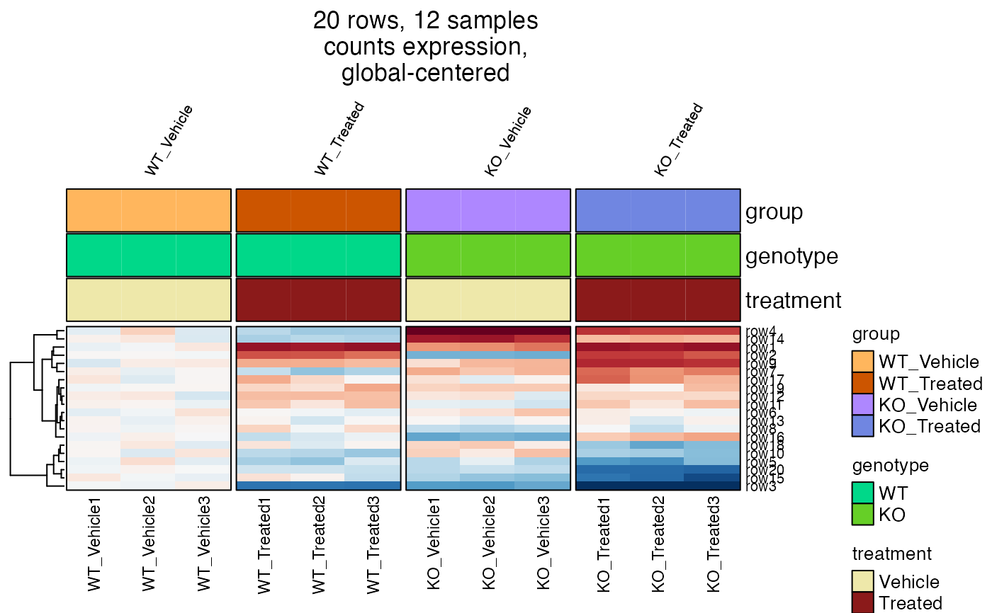
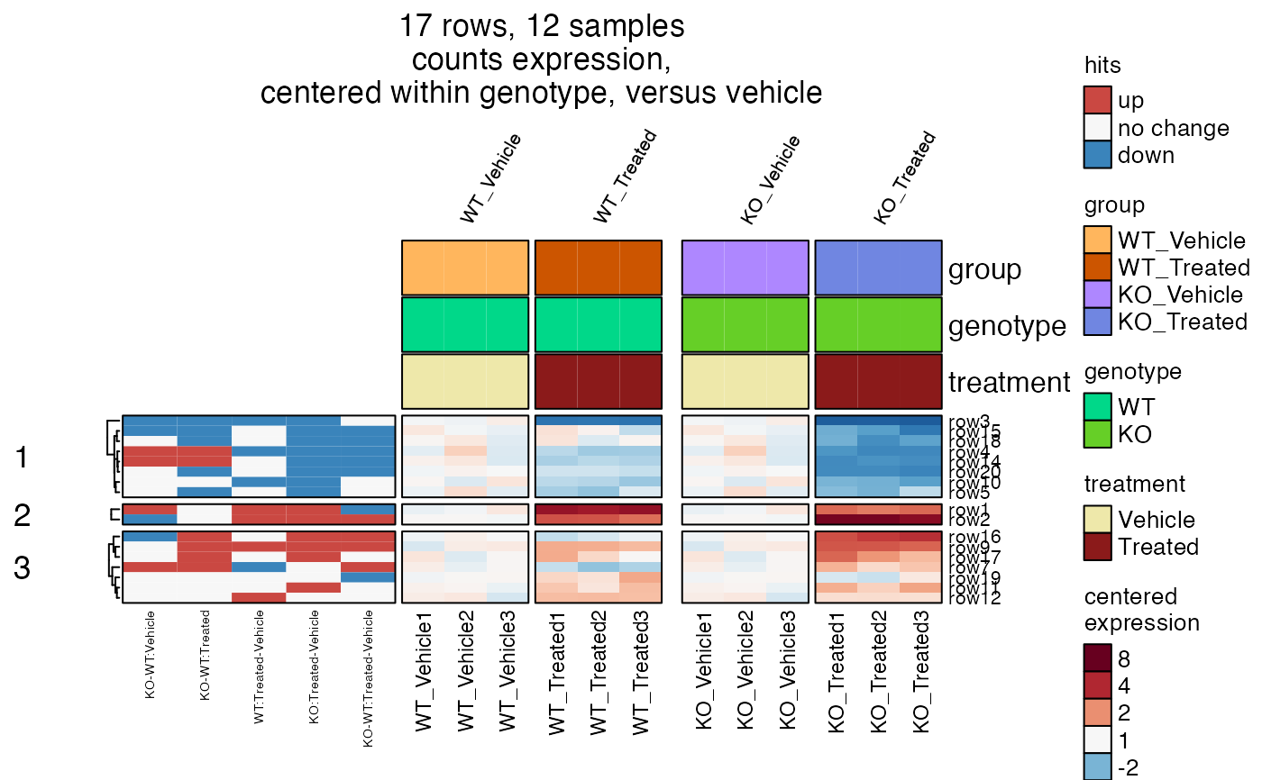
 # heatmap with hits
hm2hits <- heatmap_se(se2,
sample_color_list=sample_color_list2,
sestats=sestats2,
controlSamples=c(1:3, 7:9),
column_gap=grid::unit(c(1, 3, 1), "mm"),
control_label="versus vehicle",
centerby_colnames="genotype",
row_split=3,
row_cex=0.4,
column_title_rot=60,
column_cex=0.5,
column_title_gp=grid::gpar(fontsize=8),
column_split="group")
ComplexHeatmap::draw(hm2hits,
column_title=attr(hm2hits, "hm_title"),
merge_legends=TRUE)
# heatmap with hits
hm2hits <- heatmap_se(se2,
sample_color_list=sample_color_list2,
sestats=sestats2,
controlSamples=c(1:3, 7:9),
column_gap=grid::unit(c(1, 3, 1), "mm"),
control_label="versus vehicle",
centerby_colnames="genotype",
row_split=3,
row_cex=0.4,
column_title_rot=60,
column_cex=0.5,
column_title_gp=grid::gpar(fontsize=8),
column_split="group")
ComplexHeatmap::draw(hm2hits,
column_title=attr(hm2hits, "hm_title"),
merge_legends=TRUE)
 # venn diagram
hit_list <- hit_array_to_list(sestats2,
contrast_names=c(1:2))
jamba::sdim(hit_list);
#> rows class
#> KO_Vehicle-WT_Vehicle 8 numeric
#> KO_Treated-WT_Treated 11 numeric
# names(hit_list) <- gsub(":", ",<br>\n", contrast2comp(names(hit_list)))
# vo <- venndir::venndir(hit_list, expand_fraction=0.1)
# venndir::venndir_legender(venndir_out=vo, setlist=hit_list)
# vo <- venndir::venndir(hit_list, expand_fraction=0.1, proportional=TRUE)
# venndir::venndir_legender(venndir_out=vo, setlist=hit_list)
# venn diagram
hit_list <- hit_array_to_list(sestats2,
contrast_names=c(1:2))
jamba::sdim(hit_list);
#> rows class
#> KO_Vehicle-WT_Vehicle 8 numeric
#> KO_Treated-WT_Treated 11 numeric
# names(hit_list) <- gsub(":", ",<br>\n", contrast2comp(names(hit_list)))
# vo <- venndir::venndir(hit_list, expand_fraction=0.1)
# venndir::venndir_legender(venndir_out=vo, setlist=hit_list)
# vo <- venndir::venndir(hit_list, expand_fraction=0.1, proportional=TRUE)
# venndir::venndir_legender(venndir_out=vo, setlist=hit_list)