Multienrichment with clusterProfiler

library(multienrichjam)
#> 
library(jamba)
# library(colorjam);
# suppressPackageStartupMessages(library(ComplexHeatmap))
options("warn" = -1)

msigdbr Requirement

This guide requires the msigdbr R package from CRAN.

if (!requireNamespace("msigdbr", quietly = TRUE)) {
   jamba::printDebugHtml(
      "The ",
      "msigdbr",
      " package is required for this vignette. Stopping here."
   )
   knitr::knit_exit()
}

clusterProfiler enrichment

This document describes steps recommended for clusterProfiler enrichment data, which include specific objects such as enrichResults and others.

Refer to the clusterProfiler e-Book, an outstanding and comprehensive guide to using clusterProfiler to generate gene set enrichment data.

There are two general approaches:

1. Run clusterProfiler::enricher() for a list of experiments.
2. Use an existing list of clusterProfiler::enricher() results.

clusterProfiler enrichment

Prepare MSigDB Pathway Data

The example below demonstrates how to prepare canonical pathways from MSigDB to use for gene set enrichment. These pathways are used with a list of genes in Reese_genes to test for enrichment.

The msigdbr R package is used to download necessary data, following the guidance in the clusterProfiler e-Book: MSigDb analysis. See msigdbr::msigdbr() for more details.

Review MSigDB Collections

The msigdbr package offers convenient access to collections of gene sets available from MSigDB, shown below.

msigdb_collections <- msigdbr::msigdbr_collections(db_species = "HS")

MSigDB Collections

gs_collection	gs_subcollection	gs_collection_name	num_genesets
C1		Positional	302
C2	CGP	Chemical and Genetic Perturbations	3,538
C2	CP	Canonical Pathways	19
C2	CP:BIOCARTA	BioCarta Pathways	292
C2	CP:KEGG_LEGACY	KEGG Legacy Pathways	186
C2	CP:KEGG_MEDICUS	KEGG Medicus Pathways	658
C2	CP:PID	PID Pathways	196
C2	CP:REACTOME	Reactome Pathways	1,787
C2	CP:WIKIPATHWAYS	WikiPathways	885
C3	MIR:MIRDB	miRDB	2,377
C3	MIR:MIR_LEGACY	MIR_Legacy	221
C3	TFT:GTRD	GTRD	505
C3	TFT:TFT_LEGACY	TFT_Legacy	610
C4	3CA	Curated Cancer Cell Atlas gene sets	148
C4	CGN	Cancer Gene Neighborhoods	427
C4	CM	Cancer Modules	431
C5	GO:BP	GO Biological Process	7,583
C5	GO:CC	GO Cellular Component	1,042
C5	GO:MF	GO Molecular Function	1,855
C5	HPO	Human Phenotype Ontology	5,748
C6		Oncogenic Signature	189
C7	IMMUNESIGDB	ImmuneSigDB	4,872
C7	VAX	HIPC Vaccine Response	347
C8		Cell Type Signature	866
H		Hallmark	50

MSigDB Canonical Pathways

This tutorial uses collection = "C2" because it contains all canonical pathway gene sets from multiple sources. The canonical pathways are then filtered by retaining the subset with gs_subcollection containing "CP".

There are two columns used by clusterProfiler::enricher():

1. gs_name - the gene set name
2. gene - usually gene symbol

Using these two columns, the data.frame needs to retain only unique rows.

# C2 canonical pathways
msig_cp <- subset(
   msigdbr::msigdbr(
      species = "Homo sapiens",
      collection = "C2"
   ),
   grepl("CP", gs_subcollection)
)
msig_cp_gs <- unique(data.frame(msig_cp[, c("gs_name", "gene_symbol")]))
head(msig_cp_gs, 10)

For the purpose of this vignette, a subset of canonical pathways are available using data(msig_test), and should only be used for this analysis.

MSigDB Canonical Pathways

gs_name	gene_symbol
BIOCARTA_AGPCR_PATHWAY	ARRB1
BIOCARTA_AKAP13_PATHWAY	AKAP13
BIOCARTA_AKAP95_PATHWAY	AKAP8
BIOCARTA_AKAPCENTROSOME_PATHWAY	AKAP9
BIOCARTA_BAD_PATHWAY	ADCY1
BIOCARTA_CARM1_PATHWAY	CARM1
BIOCARTA_CASPASE_PATHWAY	APAF1
BIOCARTA_CELL2CELL_PATHWAY	ACTN1
BIOCARTA_CERAMIDE_PATHWAY	AIFM1
BIOCARTA_CFTR_PATHWAY	ADCY1

Run enricher()

The clusterProfiler documentation for enricher() is straightforward for over-representation analysis (ORA). Note that other clusterProfiler enrich* tools can be used, for example clusterProfiler::enrichKEGG(), clusterProfiler::enrichPC().

The most important argument to include:

pvalueCutoff=1

This option retains all enrichment results without filtering.
The P-value will be filtered later by multienrichjam.

This example uses Reese_genes containing genes identified by Reese et al 2019 in Epigenome-wide meta-analysis of DNA methylation and childhood asthma https://doi.org/10.1016/j.jaci.2018.11.043.

The data are stored as a list of significant genes, so we iterate the list using lapply().

# Gene hit lists
data(Reese_genes)

# enricher() for each element of a list
erlist <- lapply(Reese_genes, function(igenes) {
   er <- clusterProfiler::enricher(
      igenes,
      pvalueCutoff = 1,
      TERM2GENE = msig_test,
      minGSSize = 5,
      maxGSSize = 5000
   )
})

You may also run a specific enrichment function in clusterProfiler such as clusterProfiler::enrichPC() which automatically uses Pathway Commons pathways.

data(Reese_genes)

# Optionally run enrichPC() which tests PathwayCommons
erlist2 <- lapply(Reese_genes, function(igenes) {
   er <- clusterProfiler::enrichPC(
      igenes,
      pvalueCutoff = 1,
      minGSSize = 5,
      maxGSSize = 5000
   )
})

Run multiEnrichMap()

The erlist from the previous step will be the input to multiEnrichMap().

Mem <- multiEnrichMap(
   erlist,
   pvalueColname = "qvalue",
   p_cutoff = 0.01,
   cutoffRowMinP = 0.2,
   min_count = 2,
   topEnrichN = 20
)

The default summary for mem describes the contents, shown below:

Mem
#> class: Mem
#> dim: 2 enrichments, 14 sets, 17 genes
#> - enrichments (2): Newborns, OlderChildren
#> - sets (14): REACTOME_TAK1_DEPENDENT_IKK_AND_NF_KAPPA_B_ACTIVATION, KEGG_APOPTOSIS, ..., KEGG_ASTHMA, WP_HEAD_AND_NECK_SQUAMOUS_CELL_CARCINOMA
#> - genes (17): ACTN1, ALPK1, ..., RUNX1, SPP2
#> Analysis parameters:
#> - top N per enrichment: 20
#> - significance threshold: 0.2 (colname: qvalue)
#> - min gene count: 2
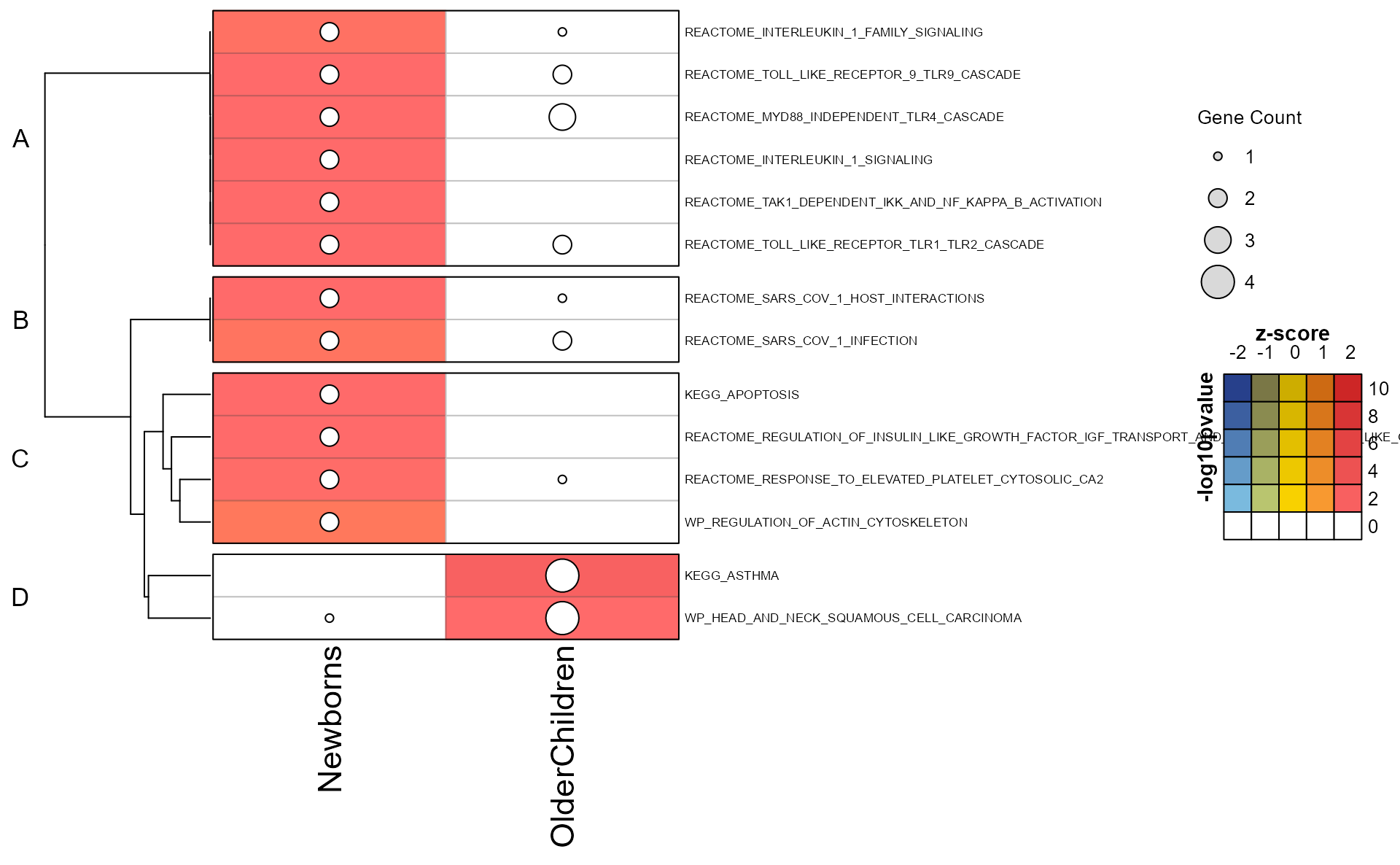
#> - direction colname: zScore

Prepare Plot Folio

The prepare_folio() represents a key step in the analysis workflow.

Pathway clusters are defined by analyst parameters:

• The number of pathways clusters
• The relative weight of the gene-pathway incidence matrix.
• The method used for clustering.

The returned MemPlotFolio provides a series of visualizations, described in detail in prepare_folio().

Mpf <- prepare_folio(
   Mem,
   pathway_column_split = 4,
   column_cex = 0.4,
   row_cex = 0.4,
   row_names_max_width = grid::unit(9, "cm"),
   column_names_max_height = grid::unit(4, "cm"),
   node_factor = 2.5,
   label_factor_l = list(
      nodeType = c(
         Set = 0.7,
         Gene = 1.5
      )
   ),
   use_shadowText = TRUE,
   main = "Canonical Pathways"
)
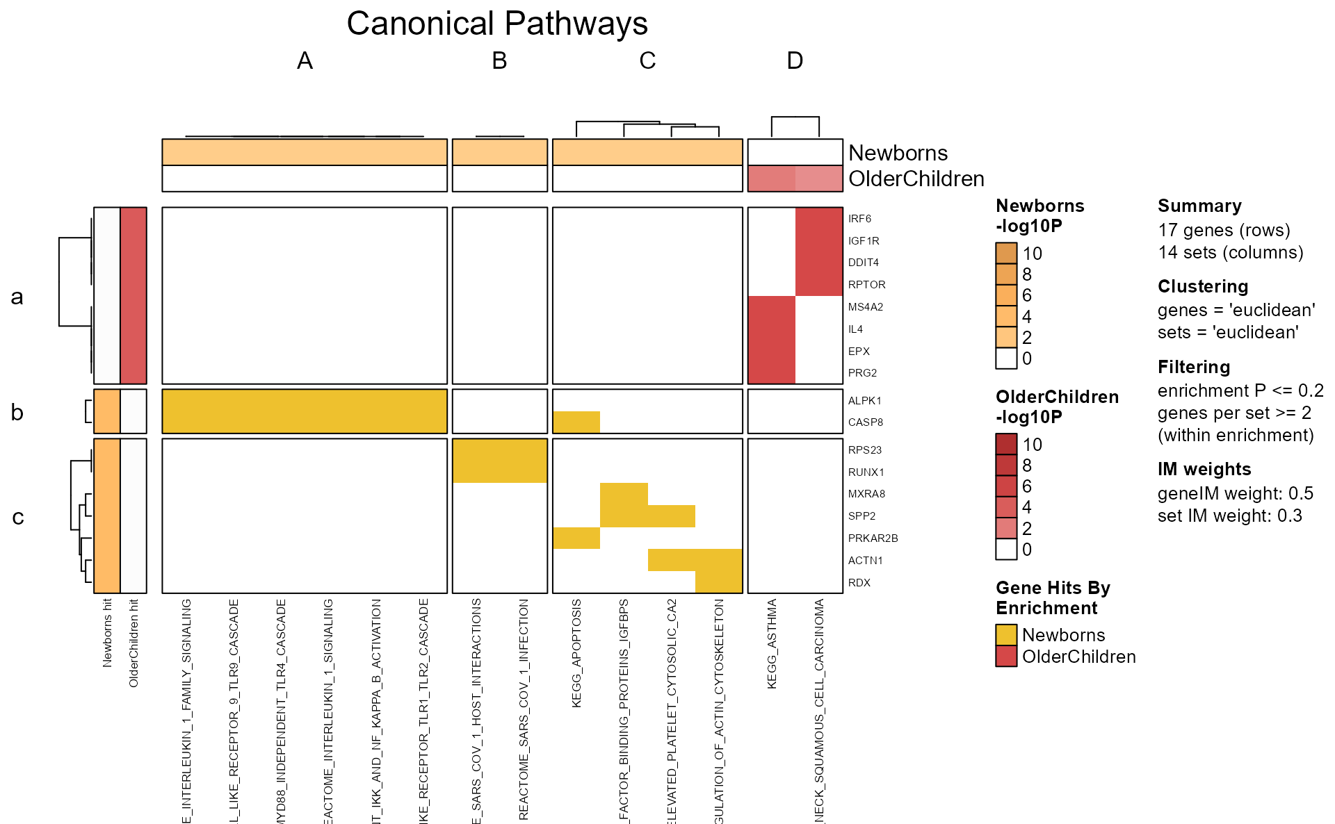
#> Loading required namespace: gridtext

Mem Plot Folio

A helper function plot_mpf() and generic function plot() both provide a convenient way to plot “all the data”.

• Use do_md_tabs='Rmd' to enable Rmarkdown HTML output to use tabs.
• Use do_md_tabs='Qmd' to enable Quarto HTML output to use tabs.

When using HTML tabs, be sure to add this chunk option: results='asis'

plot_mpf(
   Mpf,
   md_tab_level = 3,
   md_title = FALSE,
   do_md_tabs = 'Rmd',
   params = list(
      em = list(edge_factor = 0.5)
   )
)

EnrichmentHeatmap

EnrichmentMap

GenePathHeatmap

CnetCollapsed

CnetExemplar

CnetCluster

1

2

3

4

Specific Plots

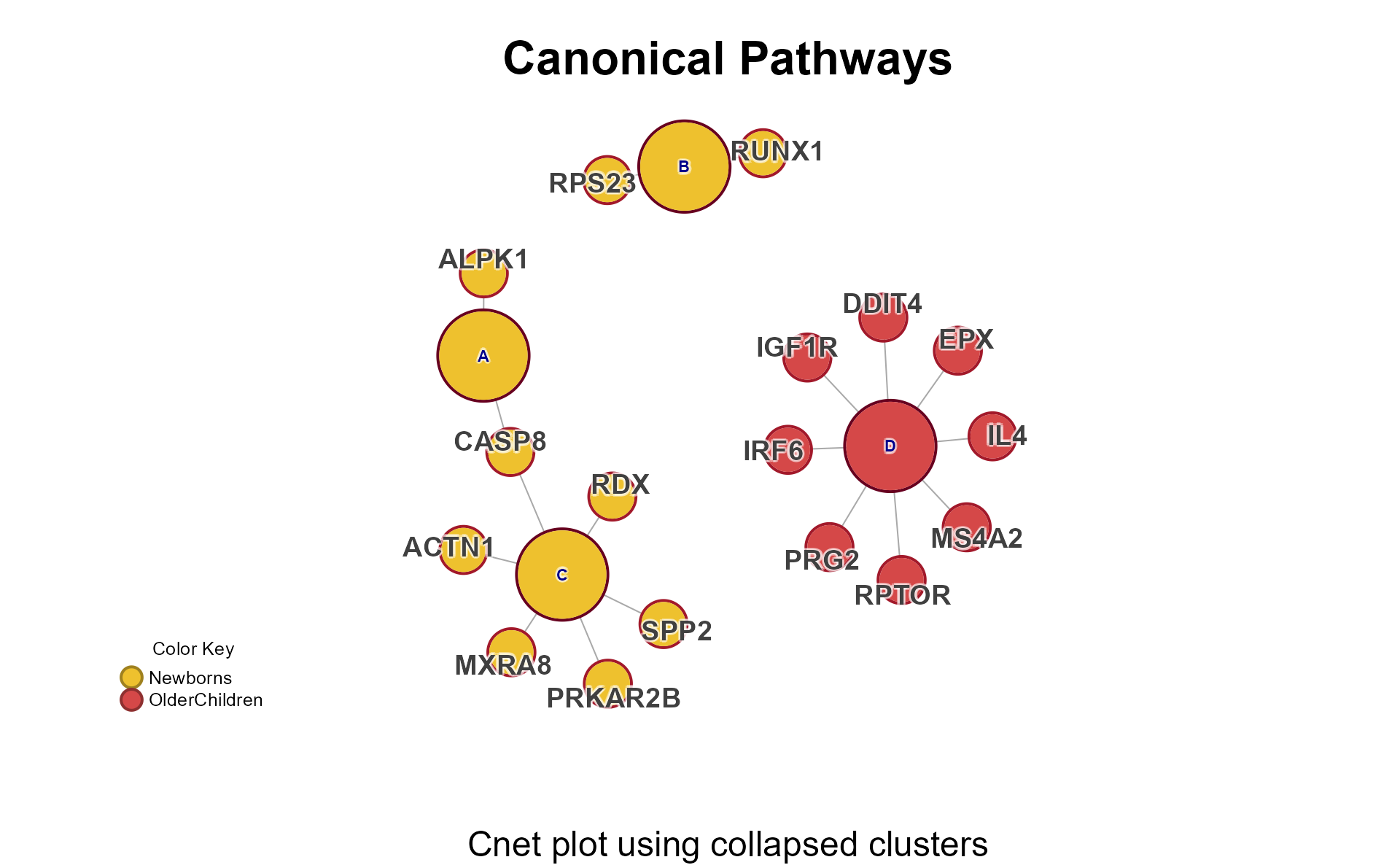
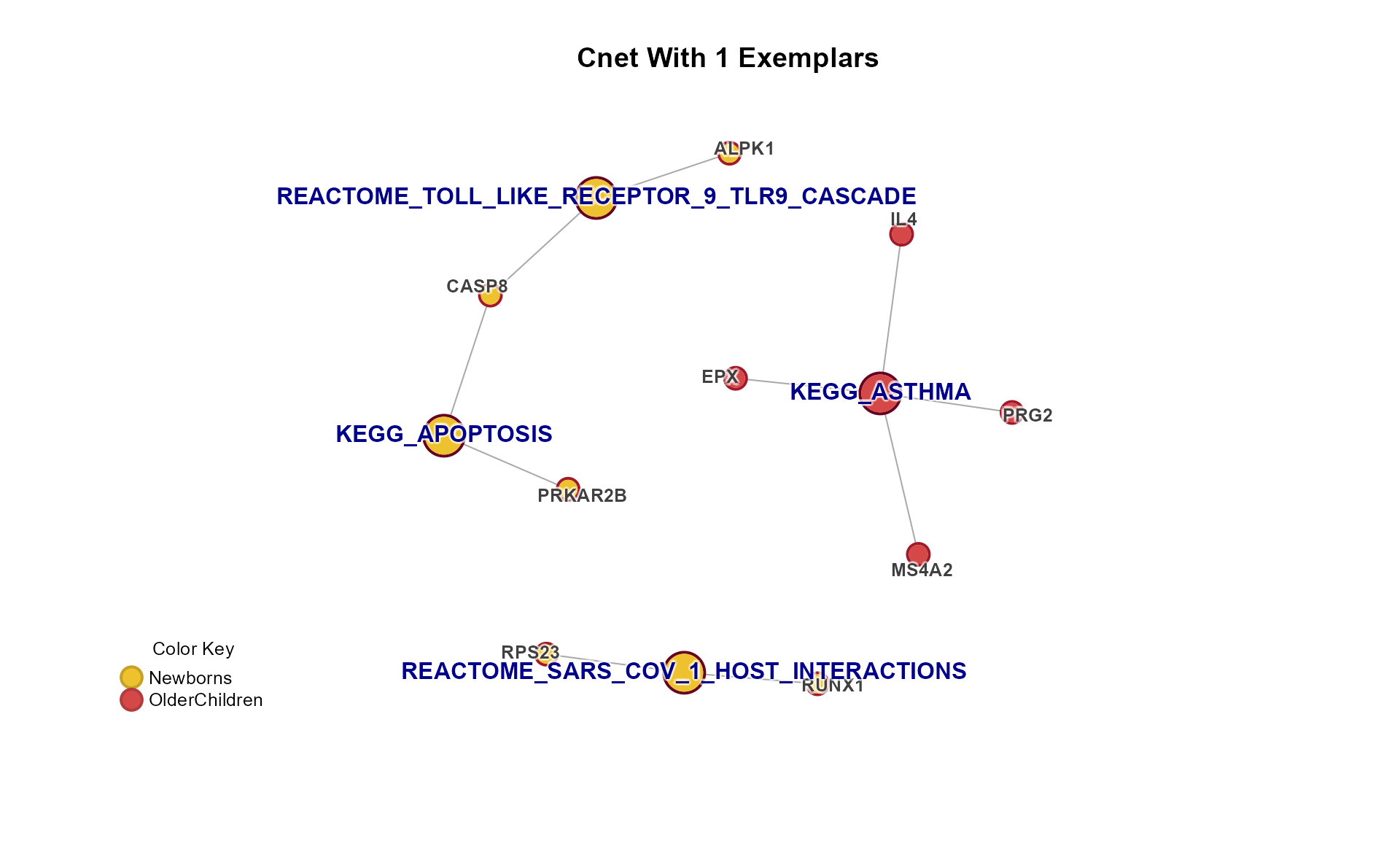
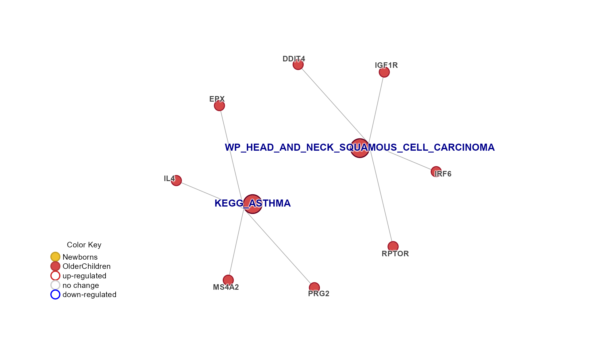
Cnet Collapsed Cluster Plot

The Cnet Collapsed Cluster Plot is often the basis for manuscript figures. The typical workflow is demonstrated below.

• cnet <- CnetCollapsed(mpf, type="set") retrieves the Cnet igraph object.
• do_plot = FALSE does not plot the Cnet network just yet.

# extract the cnet
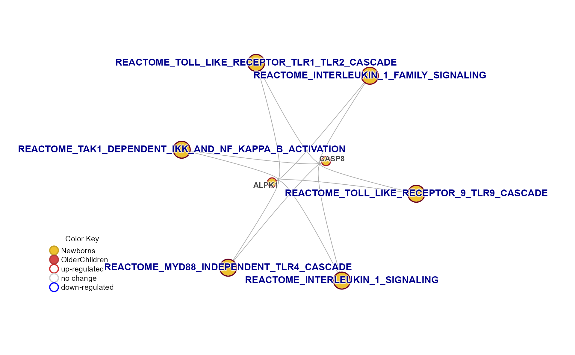
cnet <- CnetCollapsed(Mpf, do_plot = FALSE, type = "cluster")

jam_igraph() is a custom plotting function with enhancements:

• node_factor = 2 multiplies node size by 2.
• label_dist_factor = 2 multiplies label distance from node center by 5.
• use_shadowText = TRUE uses shadowing around the text labels.
• label_factor_l resizes the node labels by ‘nodeType’ for Gene and Set.
• It applies edge bundling, which helps with large networks.
• It plots using vectorized optimization.

# jam_graph instead of plot()
jam_igraph(
   cnet,
   node_factor = 2,
   use_shadowText = TRUE,
   label_dist_factor = 5,
   label_factor_l = list(
      nodeType = c(
         Gene = 2,
         Set = 1
      )
   )
)

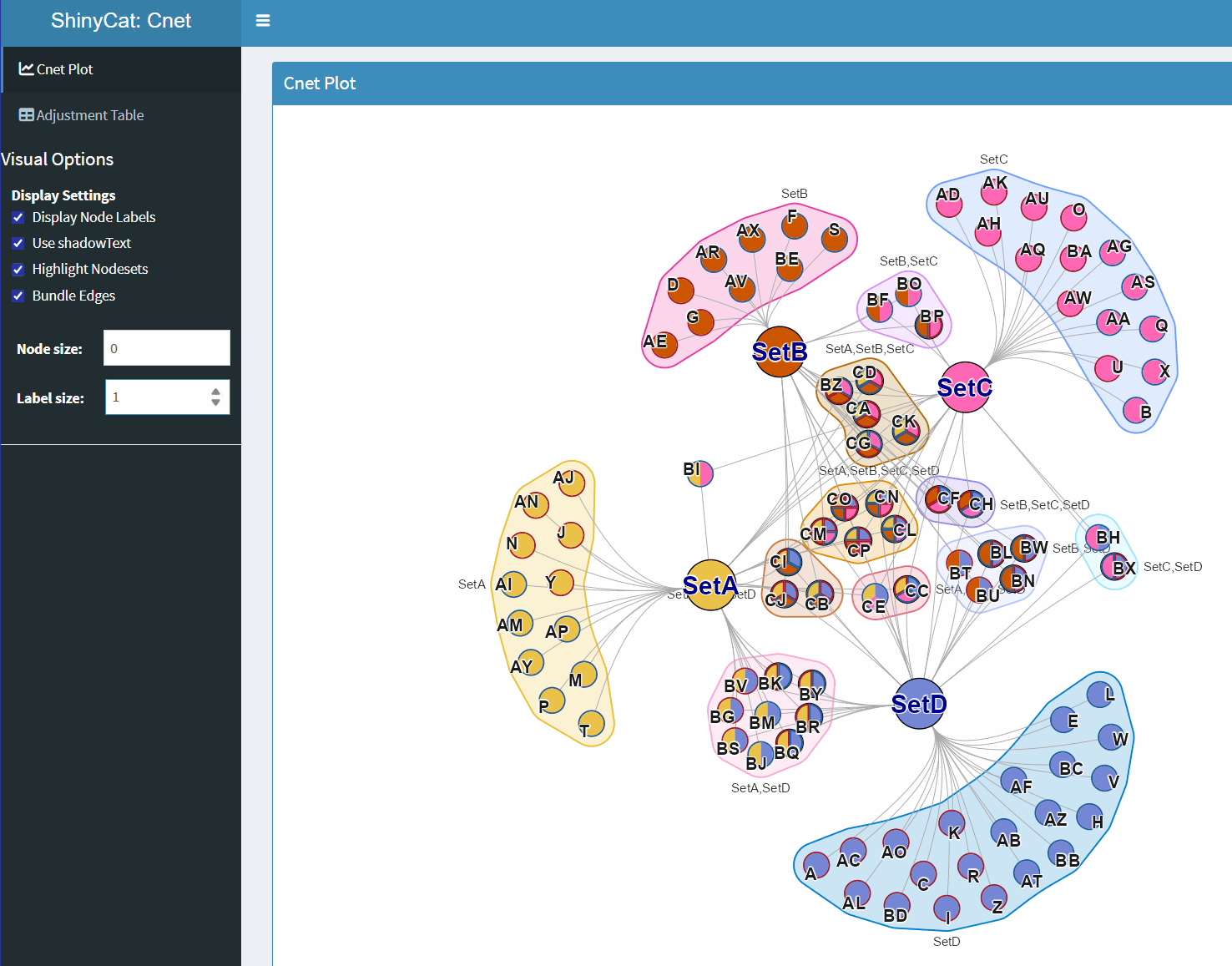
ShinyCat for Custom Cnet Layout

The R-shiny Cnet Adjustment Tool ShinyCat is intended to help polish the Cnet plot layout when making a final figure.

The R-shiny app uses several functions:

• nudge_igraph_node(): mode individual nodes
• adjust_cnet_nodeset(): adjust spacing, position, rotation of a nodeset
• reorder_igraph_nodes(): sort nodes in a group by color
• spread_igraph_labels(): arrage labels radially away from incoming edges
• bulk_cnet_adjustments(): several operations applied in bulk

Make sure to assign the output to a variable, or to click “Save RData” from within the R-shiny app. For example:

output_env <- launch_shinycat(g = cnet)

The output is stored in an environment called output_env.

# obtain the output data
adj_cnet <- output_env$adj_cnet

Then the new Cnet plot can be plotted, for example:

# jam_graph
jam_igraph(
   adj_cnet,
   node_factor = 2,
   use_shadowText = TRUE,
   label_factor_l = list(nodeType = c(Gene = 2, Set = 1))
)

ShinyCat Screenshot

An example of ShinyCat in action is shown below.