MA-plots using ggplot2
ggjammaplot(
  x,
  nbin_factor = 1,
  bw_factor = 1,
  assay_name = 1,
  useMedian = FALSE,
  controlSamples = NULL,
  centerGroups = NULL,
  colramp = c("transparent", "lightblue", "blue", "navy", "orange", "orangered2"),
  groupedX = TRUE,
  grouped_mad = TRUE,
  outlierMAD = 5,
  mad_row_min = 4,
  displayMAD = FALSE,
  noise_floor = 0,
  noise_floor_value = NA,
  naValue = NA,
  centerFunc = centerGeneData,
  whichSamples = NULL,
  useRank = FALSE,
  titleBoxColor = "lightgoldenrod1",
  outlierColor = "lemonchiffon",
  fillBackground = TRUE,
  maintitle = NULL,
  subtitle = NULL,
  summary = "mean",
  difference = "difference",
  transFactor = 0.2,
  doPlot = TRUE,
  highlightPoints = NULL,
  highlightPch = 21,
  highlightCex = 1.5,
  highlightColor = NULL,
  doHighlightLegend = TRUE,
  ablineH = c(-2, 0, 2),
  base_size = 12,
  panel.grid.major.colour = "grey90",
  panel.grid.minor.colour = "grey95",
  return_type = c("ggplot", "data"),
  xlim = NULL,
  ylim = c(-6, 6),
  ncol = NULL,
  nrow = NULL,
  blankPlotPos = NULL,
  verbose = FALSE,
  ...
)
Arguments
- x
one of the following inputs:
numericmatrixSummarizedExperimentobject, where the assay data is defined usingassays(x)[[assay_name]]. Accordingly,assay_namecan be either an integer index orcharacterstring matching thenames(assays(x)).listoutput fromjammacalc()orjammaplot(), where each element in the list is a two-columnmatrixwith colnamesc("x", "y").
- nbin_factor
numericvalue used to adjust the number of bins used to display the MA-plots, where values higher than1increase the resolution and level of detail, and values below1decrease the resolution. Note the number of bins are already adjusted based upon the square root of the number of plot panels, andnbin_factorapplied to that value.- bw_factor
numericused to adjust the resolution of the 2-dimensional bandwidth calculation, where higher values create more detailed density, and lower values create a smoother density across the range of data.- assay_name
relevant only when
xisSummarizedExperiment, one of these input types:characterstring that matchesnames(assays(x))integerindex forassays(x), where any value higher thanlength(assays(x))is adjusted tolength(assays(x)), which makes it convenient to select the last element in the list ofassays(x)by usingassay_name = Inf.
- useMedian
logicalindicating whether calculations should usemedian, or whenuseMedian=FALSEthemeanis used. The median has the benefit of reducing effect of outliers, however the mean has the advantage that it represents data consistent with most parametric statistical analyses.- controlSamples
charactervector ofcolnames(x)to use as the control when calculating centered data. By default, all samples are used, so the classic MA-plot is the value of each sample, subtracting the median or mean value calculated across all samples. It is sometimes useful to define a subset of known samples for this calculation, which can be beneficial in avoiding outliers, or for consistency by selecting high quality control samples.- centerGroups
charactervector with length equal toncol(x), which defines subgroups ofcolnames(x)to be treated independently during the MA-plot calculation.- colramp
one of several inputs recognized by
jamba::getColorRamp(). It typically recognizes either the name of a color ramp from RColorBrewer, the name of functions from theviridispackage such asviridis::viridis(), or single R colors, or a vector of R colors. When a single color is supplied, a gradient is created from white to that color, where the default base color can be customized withdefaultBaseColor="black"for example.- groupedX
logicalindicating whether the x-axis value, which represents the median or mean value, should be calculated independently for each group whencenterGroupsis used with multiple groups. TypicallygroupedX=TRUEis recommended, however it can be beneficial to share an overall x-axis value in specific circumstances.- grouped_mad
logicalindicating whether the MAD factor calculation of variability among samples should be performed independently for each group whencenterGroupsis used with multiple groups. Typicallygrouped_max=TRUEis recommended, however it can be beneficial to share an overall MAD factor threshold across all samples in specific circumstances.- outlierMAD
numericindicating the MAD factor threshold above which a particular sample is considered an outlier.- mad_row_min
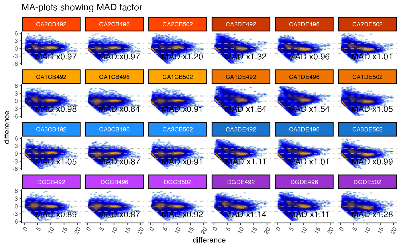
numericvalue indicating the minimum x-axis value, calculated using either median or mean as defined by argumentuseMedian, at or above which a measurement is used in the MAD factor calculation. This threshold is useful to restrict the MAD variability calculation to measurements (rows inx) with signal that meets a minimum noise threshold.- displayMAD
logicalindicating whether to display the MAD factor in the bottom right corner of each MA-plot panel.- noise_floor, noise_floor_value
numericto define a numeric floor, orNULLfor no numeric floor. Values at or belownoise_floorare set tonoise_floor_value, intended for two potential uses:Filter out value below a threshold, so they do not affect centering.
This option is valuable to remove zeros when a zero
0is considered "no measurement observed", typically for count data such as RNA-seq, NanoString, and especially single-cell protocols or other protocols that produce a large number of missing values.One can typically tell whether input data includes zero
0values by the presence of characteristic 45-degree angle lines originating fromx=0angled toward the right. The points along this line are rows with more measurements of zero than non-zero, there this sample has a non-zero value.
Set values at a noise floor to the noise floor, to retain the measurement but minimize the effect during centering to the lowest realiable measurement for the platform technology.
This value may be set to a platform noise floor for something like microarray data where the intensity may be unreliable below a threshold; or
for quantitative PCR measurements where cycle threshold (Ct) values may become unreliable, for example above CT=40 or CT=35. Data is often transformed to abundance with
2 ^ (40 - CT)then log2-transformed for analysis. In this case, to apply anoise_flooreffective for CT=35, one would usenoise_floor=5.
- naValue
characterstring used to convert values ofNAto something else. This argument is useful when a numeric matrix may containNAvalues but would prefer them to be, for example,0.- centerFunc
functionused to supply a custom data centering function. In practice this argument should rarely be changed.- whichSamples
integerindex of samples incolnames(x)to be plotted, however all samples incolnames(x)will be used for the MA-plot calculations and data centering. This argument is intended to help zoom in to inspect a specific subset of samples, without having to plot all samples inx.- useRank
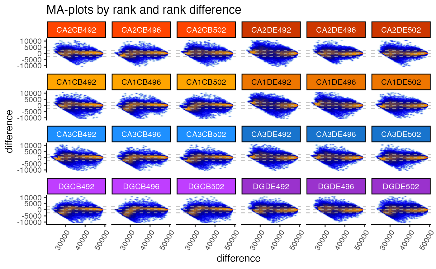
logicalindicating whether to plot rank on the x-axis, rank-difference on the y-axis for each sample. This transformation is rather useful, especially when downstream analysis tools may also refer to the rank value of particular measurements.- titleBoxColor
charactervector of R colors, wheretitleBoxColoris equal toncol(x), or wherenames(titleBoxColor)matchescolnames(x). When supplied, each plot panel strip background will be colored accordingly.- outlierColor
characterstring representing one R color, used whencolrampOutlierisNULLand whenoutlierMADis defined. This color is used for MA-plot outlier panels by substituting the first color from thecolrampcolor ramp, to act as a visual cue that the panel represents an outlier.- fillBackground
logicalcurrently used for base R graphics output, and passed tojamba::plotSmoothScatter(), indicating whether to fill the plot panel using the first color in the color ramp for each MA-plot panel, or when a plot panel is an outlier, it usesoutlierColor. This argument is mainly useful to highlight outlier panels, although it is also useful when the color ramp has non-white base color, for exampleviridis::viridis().- maintitle
characterstring with the title displayed above all individual MA-plot panels. It will appear in the top outer margin.- subtitle
NULLorcharactervector to be drawn at the bottom left corner of each plot panel, the location is defined bysubtitlePreset.- transFactor
numericadjustment to the visual density of smooth scatter points. For base R graphics, this argument is passed tojamba::plotSmoothScatter(). The argument value is based upongraphics::smoothScatter()argumenttransformation, which uses defaultfunction(x)x^0.25. ThetransFactoris equivalent to the exponential in the form:function(x)x^transFactor. Lower values make the point density more visually intense, higher values make the point density less visually intense.- doPlot
logicalindicating whether to create plots. WhendoPlot=FALSEonly the MA-plot panel data is returned.- highlightPoints
NULL, orcharactervector, or alistofcharactervectors indicatingrownames(x)to highlight in each MA-plot panel. WhenNULL, no points are highlighted; whencharactervector, points are highlighted in all MA-plot panels; whenlistofcharactervectors, eachcharactervector in the list is highlighted using a unique color inhighlightColor. Points are drawn usinggraphics::points()and colored usinghighlightColor, which can be time-consuming for a large number of highlight points.- highlightCex
numericvalue recycled tolength(highlightPoints)indicating the highlight point size.- highlightColor
charactervector used whenhighlightPointsis defined. It is recycled tolength(highlightPoints)and is applied either to- doHighlightLegend
logicalindicating whether to print a color legend whenhighlightPointsis defined. The legend is displayed in the bottom outer margin of the page usingouter_legend(), and the page is adjusted to add bottom outer margin.- ablineH
numericvector indicating position of horizontal and vertical lines in each MA-plot panel.- xlim
NULLornumericvectorlength=2indicating the y-axis and x-axis ranges, respectively. The values are useful to define consistent dimensions across all panels. The defaultylim=c(-4,4)represents 16-fold up and down range in normal space, and is typically a reasonable starting point for most purposes. Even if numeric values are all between-1.5and1.5, it is still recommended to keep a range in context ofc(-4, 4), to indicate that the observed values are lower than typically observed. Thec(-4, 4)may be adjusted relative to the typical ranges expected for the data. It is sometimes helpful to definexlimslightly above zero for datasets that have an extremely large proportion of zeros, in order to reduce the visual effect of having that much point density at zero, for example withxlim=c(0.001, 20)andapplyRangeCeiling=FALSE.- ylim
NULLornumericvectorlength=2indicating the y-axis and x-axis ranges, respectively. The values are useful to define consistent dimensions across all panels. The defaultylim=c(-4,4)represents 16-fold up and down range in normal space, and is typically a reasonable starting point for most purposes. Even if numeric values are all between-1.5and1.5, it is still recommended to keep a range in context ofc(-4, 4), to indicate that the observed values are lower than typically observed. Thec(-4, 4)may be adjusted relative to the typical ranges expected for the data. It is sometimes helpful to definexlimslightly above zero for datasets that have an extremely large proportion of zeros, in order to reduce the visual effect of having that much point density at zero, for example withxlim=c(0.001, 20)andapplyRangeCeiling=FALSE.- ncol
integernumber of MA-plot panel columns and rows passed tographics::par("mfrow")whendoPar=TRUE. When only one value is supplied,nroworncol, the other value is defined byncol(x)andblankPlotPosso all panels can be contained on one page. Whennrowandncolare defined such that multiple pages are produced, each page will be annotated withmaintitleanddoHighlightLegendas relevant.- nrow
integernumber of MA-plot panel columns and rows passed tographics::par("mfrow")whendoPar=TRUE. When only one value is supplied,nroworncol, the other value is defined byncol(x)andblankPlotPosso all panels can be contained on one page. Whennrowandncolare defined such that multiple pages are produced, each page will be annotated withmaintitleanddoHighlightLegendas relevant.- blankPlotPos
NULLorintegervector indicating plot panel positions to be drawn blank, and therefore skipped. Plot panels are drawn in the exact order ofcolnames(x)received. Blank panel positions are intended to help customize the visual alignment of MA-plot panels. The mechanism is similar toggplot2::facet_wrap()except that blank positions can be manually defined by what makes sense for the experiment design.- verbose
logical indicating whether to print verbose output.
- ...
additional parameters sent to downstream functions,
jamba::plotSmoothScatter,centerGeneData.
Details
This method is under active development and may change as features are implemented.
It is currently fully functional and is being documented.
See also
Other jam plot functions:
jammaplot()
Examples
if (jamba::check_pkg_installed("SummarizedExperiment") &&
jamba::check_pkg_installed("farrisdata")) {
suppressPackageStartupMessages(require(SummarizedExperiment));
GeneSE <- farrisdata::farrisGeneSE;
titleBoxColor <- jamba::nameVector(
farrisdata::colorSub[as.character(colData(GeneSE)$groupName)],
colnames(GeneSE));
options("warn"=FALSE);
gg <- ggjammaplot(GeneSE,
ncol=6,
base_size=12,
assay_name="raw_counts")
gg <- ggjammaplot(GeneSE,
ncol=6,
assay_name="counts",
useRank=TRUE,
ylim=c(-11000, 11000),
maintitle="MA-plots by rank and rank difference",
titleBoxColor=titleBoxColor)
gg <- ggjammaplot(GeneSE,
ncol=6,
assay_name="counts",
titleBoxColor=titleBoxColor,
base_size=10,
maintitle="MA-plots showing MAD factor",
displayMAD=TRUE)
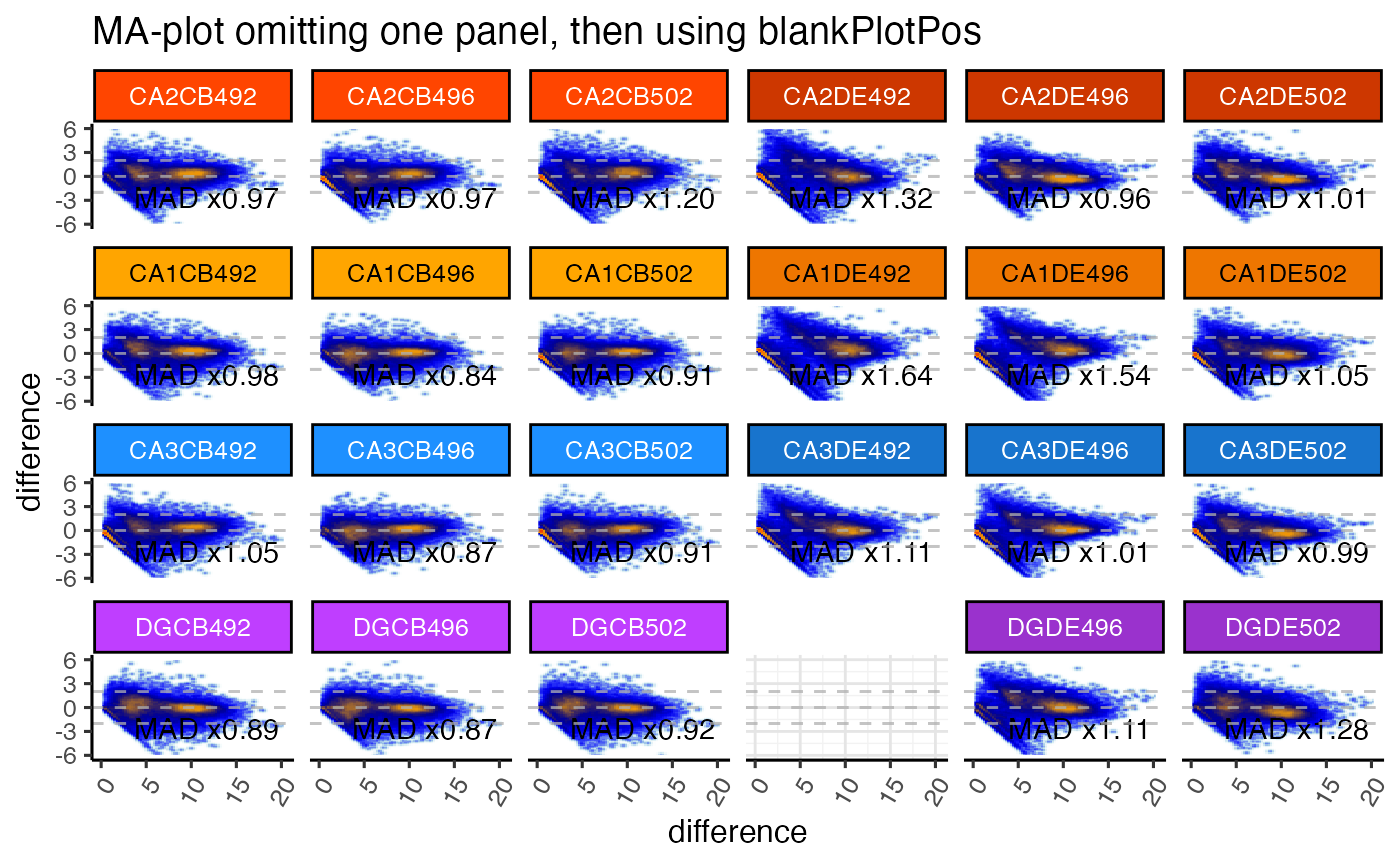
gg <- ggjammaplot(GeneSE,
ncol=6,
assay_name="counts",
titleBoxColor=titleBoxColor,
maintitle="MA-plot omitting one panel, then using blankPlotPos",
whichSamples=colnames(GeneSE)[c(1:21, 23:24)],
blankPlotPos=22,
displayMAD=TRUE)
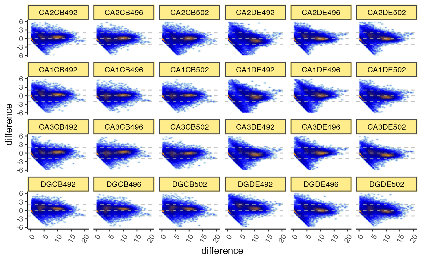
if (FALSE) {
ggdf <- ggjammaplot(GeneSE,
assay_name="counts",
whichSamples=c(1:3, 7:9),
return_type="data",
titleBoxColor=titleBoxColor)
highlightPoints1 <- names(jamba::tcount(subset(ggdf, mean > 15 & difference < -1)$item, 2))
highlightPoints2 <- subset(ggdf, name %in% "CA1CB492" &
difference < -4.5)$item;
highlightPoints <- list(
divergent=highlightPoints1,
low_CA1CB492=highlightPoints2);
ggdf_h <- ggjammaplot(GeneSE,
assay_name="counts",
highlightPoints=highlightPoints,
whichSamples=c(1:3, 7:9),
return_type="data",
titleBoxColor=titleBoxColor)
# you can use output from `jammaplot()` as input to `ggjammaplot()`:
jp2 <- jammaplot(GeneSE,
outlierMAD=2,
doPlot=FALSE,
assay_name="raw_counts",
filterFloor=1e-10,
filterFloorReplacement=NA,
centerGroups=colData(GeneSE)$Compartment,
subtitleBoxColor=farrisdata::colorSub[as.character(colData(GeneSE)$Compartment)],
useRank=FALSE);
gg1 <- ggjammaplot(jp2,
ncol=6,
titleBoxColor=titleBoxColor);
print(gg1);
}
}
#> Warning: package ‘SummarizedExperiment’ was built under R version 3.6.2
#> Warning: package ‘S4Vectors’ was built under R version 3.6.3
#> Warning: package ‘IRanges’ was built under R version 3.6.2
#> Warning: package ‘GenomeInfoDb’ was built under R version 3.6.3
#> Warning: package ‘DelayedArray’ was built under R version 3.6.3
#> Warning: package ‘matrixStats’ was built under R version 3.6.2
#> Warning: package ‘BiocParallel’ was built under R version 3.6.2
#> Warning: Ignoring unknown parameters: stat
#> Warning: Removed 534 rows containing non-finite values (stat_density2d).
#> Warning: Removed 7776 rows containing missing values (geom_raster).
#> Warning: Ignoring unknown parameters: stat
 #> Warning: Removed 140 rows containing non-finite values (stat_density2d).
#> Warning: Removed 7776 rows containing missing values (geom_raster).
#> Warning: Ignoring unknown parameters: stat
#> Warning: Removed 140 rows containing non-finite values (stat_density2d).
#> Warning: Removed 7776 rows containing missing values (geom_raster).
#> Warning: Ignoring unknown parameters: stat
 #> Warning: Removed 322 rows containing non-finite values (stat_density2d).
#> Warning: Removed 7776 rows containing missing values (geom_raster).
#> Warning: Ignoring unknown parameters: stat
#> Warning: Removed 322 rows containing non-finite values (stat_density2d).
#> Warning: Removed 7776 rows containing missing values (geom_raster).
#> Warning: Ignoring unknown parameters: stat
 #> Warning: Removed 317 rows containing non-finite values (stat_density2d).
#> Warning: Removed 7636 rows containing missing values (geom_raster).
#> Warning: Removed 317 rows containing non-finite values (stat_density2d).
#> Warning: Removed 7636 rows containing missing values (geom_raster).