Splicejam basic RNAseq workflow
James M. Ward
2021-03-09
Source:vignettes/basic-rnaseq-workflow.Rmd
basic-rnaseq-workflow.RmdThis vignette is intended to demonstrate the basic analysis workflow for RNA-seq data.
Salmon “quant.sf.gz” files
This example begins with Salmon quantification files from the tximportData package (if available).
if (suppressPackageStartupMessages(require(tximportData))) {
   dir <- system.file("extdata", package="tximportData");

   # read sample annotations as a data.frame
   samples <- read.table(file.path(dir, "samples.txt"), header=TRUE);
   samples;

   # define Salmon import files
   files <- jamba::nameVector(file.path(dir, "salmon", samples$run, "quant.sf.gz"),
      samples$run);
   data.frame(files);
}
#>                                                                                           files
#> ERR188297 /Users/wardjm/Library/R/3.6/library/tximportData/extdata/salmon/ERR188297/quant.sf.gz
#> ERR188088 /Users/wardjm/Library/R/3.6/library/tximportData/extdata/salmon/ERR188088/quant.sf.gz
#> ERR188329 /Users/wardjm/Library/R/3.6/library/tximportData/extdata/salmon/ERR188329/quant.sf.gz
#> ERR188288 /Users/wardjm/Library/R/3.6/library/tximportData/extdata/salmon/ERR188288/quant.sf.gz
#> ERR188021 /Users/wardjm/Library/R/3.6/library/tximportData/extdata/salmon/ERR188021/quant.sf.gz
#> ERR188356 /Users/wardjm/Library/R/3.6/library/tximportData/extdata/salmon/ERR188356/quant.sf.gz
Transcript-to-gene from GTF
The transcript-to-gene association will be stored in a data.frame tx2geneDF, in this case using splicejam::makeTx2geneFromGtf(). For other ways of creating a tx2gene data.frame, see the vignette from the tximport::tximport package.
For the purpose of this example, the GTF file is used from the tximportData package (if available).
if (suppressPackageStartupMessages(require(tximportData))) {
   gtfFile <- head(
      list.files(pattern="gtf.gz",
         path=system.file("extdata/salmon_dm", package="tximportData"),
         full.names=TRUE),
      1);
   gtfFile;
   tx2geneDF <- makeTx2geneFromGtf(GTF=gtfFile);
   txColname <- "transcript_id";
   geneColname <- "gene_name";
   print(head(tx2geneDF));

   ## Alternatively, we load a prepared file from tximportData
   tx2geneDF <- data.table::fread(
      file.path(dir, "tx2gene.gencode.v27.csv"),
      sep=",",
      data.table=FALSE);
   txColname <- colnames(tx2geneDF)[1];
   geneColname <- colnames(tx2geneDF)[2];
}
#>                 gene_id      gene_name transcript_id
#> FBtr0081624 FBgn0000003 7SLRNA:CR32864   FBtr0081624
#> FBtr0342981 FBgn0000008              a   FBtr0342981
#> FBtr0071763 FBgn0000008              a   FBtr0071763
#> FBtr0100521 FBgn0000008              a   FBtr0100521
#> FBtr0071764 FBgn0000008              a   FBtr0071764
#> FBtr0306337 FBgn0000014          abd-A   FBtr0306337
Import Salmon transcript data
In this case, Salmon quantification files are imported, via the tximport package (if available).
A summary of imported data is shown using the function jamba::sdim() which prints the dimensions of each object in a list.
if (suppressPackageStartupMessages(require(tximportData)) &&
      suppressPackageStartupMessages(require(tximport))) {
   txiTx <- tximport::tximport(files,
      type="salmon",
      txOut=TRUE);

   ## Check the data returned
   jamba::sdim(txiTx);
}
#> reading in files with read_tsv
#> 1 2 3 4 5 6
#>                       rows cols     class
#> abundance           200401    6    matrix
#> counts              200401    6    matrix
#> length              200401    6    matrix
#> countsFromAbundance      1      character
SummarizedExperiment for transcript data
It is helpful and consistent with other Bioconductor workflows to use a commonly-used object "SummarizedExperiment". This object stores gene data, biological sample data, and one or more data matrices containing assay data (measurements) in one convenient object.
Note: During this step, data is log2-transformed using the format
log2(1+x).
## Create SummarizedExperiment transcript object
if (suppressPackageStartupMessages(require(SummarizedExperiment)) &&
      exists("txiTx")) {

   assayNames <- intersect(c("abundance","counts"),
      names(txiTx));
   geneMatch <- match(rownames(txiTx[[assayNames[1]]]),
      tx2geneDF[,txColname]);
   sampleDF <- data.frame(
      Sample=colnames(txiTx[[assayNames[1]]]),
      Group=rep(c("A", "B"),
         length.out=ncol(txiTx[[assayNames[1]]])));

   TxSE <- SummarizedExperiment(
      assays=lapply(txiTx[assayNames], function(x){log2(1+x)}),
      rowData=DataFrame(tx2geneDF[geneMatch,,drop=FALSE]),
      colData=DataFrame(sampleDF)
   );
}
Import Salmon gene data using tx2geneDF
If data were imported at the transcript level (above) then it can be summarized at the gene level without re-importing from the source files. Alternatively, it can be imported from source files without importing at the transcript level. Both methods are shown below.
##
if (suppressPackageStartupMessages(require(tximportData))) {
   if (exists("txiTx")) {
      ## Summarize transcript data to the gene level
      txiGene <- tximport::summarizeToGene(txiTx,
         tx2gene=tx2geneDF[,c(txColname,geneColname)]);
   } else {
      ## Import Salmon data and summarize to genes directly
      txiGene <- tximport::tximport(unname(files),
         type="salmon",
         tx2gene=tx2geneDF[,c(txColname,geneColname)]);
   }

   ## Check the data returned
   jamba::sdim(txiGene);
}
#> summarizing abundance
#> summarizing counts
#> summarizing length
#>                      rows cols     class
#> abundance           58288    6    matrix
#> counts              58288    6    matrix
#> length              58288    6    matrix
#> countsFromAbundance     1      character
SummarizedExperiment for gene data
It is helpful and consistent with other Bioconductor workflows to use a commonly-used object “SummarizedExperiment”. This object stores gene data, biological sample data, and one or more data matrices in one convenient format.
Note: This step is a convenient time to annotate the gene data.frame, for example the steps below will use gene-related
colnames(tx2geneDF)where possible. If a “gene_name” or “gene_symbol” colname does not exist, this step would be a good time to add that data.
Note: During this step, data is log2-transformed using the format
log2(1+x).
## Create SummarizedExperiment transcript object
if (exists("txiGene")) {
   assayNamesG <- intersect(c("abundance","counts"), names(txiGene));
   geneMatchG <- match(rownames(txiGene[[assayNames[1]]]),
      tx2geneDF[,geneColname]);
   geneColnames <- unique(c(geneColname,
      jamba::unvigrep("^trans|^tx", colnames(tx2geneDF))));

   sampleDF <- data.frame(Sample=colnames(txiGene[[assayNames[1]]]),
      Group=rep(c("A", "B"), length.out=ncol(txiGene[[assayNames[1]]])));

   GeneSE <- SummarizedExperiment(
      assays=lapply(txiGene[assayNamesG], function(x){log2(1+x)}),
      rowData=DataFrame(tx2geneDF[geneMatchG,geneColnames,drop=FALSE]),
      colData=DataFrame(sampleDF)
   )
}
Transcript-level analysis steps
Define detected transcripts
Often the RNA-seq data includes a number of transcripts for which there is no detectable signal. Several filtering methods are encapsulated into a function defineDetectedTx() to filter transcript isoform data which should be considered below the effective limit of detection.
At this step, group mean values are used for filtering, however it can be performed without grouping, by setting groups=colnames(TxSE).
if (exists("TxSE")) {
   cutoffTxExpr <- 7;
   cutoffTxTPMExpr <- 1;
   cutoffTxPctMax <- 10;
   detectedTxTPML <- defineDetectedTx(
      iMatrixTx=assays(TxSE)[["counts"]],
      iMatrixTxTPM=assays(TxSE)[["abundance"]],
      groups=nameVector(colData(TxSE)$Group, colnames(TxSE)),
      cutoffTxPctMax=cutoffTxPctMax,
      cutoffTxExpr=cutoffTxExpr,
      cutoffTxTPMExpr=cutoffTxTPMExpr,
      tx2geneDF=renameColumn(rowData(TxSE),
        from=c(geneColname,txColname),
        to=c("gene_name","transcript_id")),
      useMedian=FALSE,
      verbose=FALSE);
   detectedTx <- detectedTxTPML$detectedTx;
   numDetectedTx <- length(detectedTx);
   detectedGenes <- mixedSort(unique(rowData(TxSE[detectedTx,])[,geneColname]));
   numDetectedGenes <- length(detectedGenes);
   jamba::printDebug("Defined ",
      format(big.mark=",", numDetectedTx),
      " detected Tx representing ",
      format(big.mark=",", numDetectedGenes),
      " genes.");
}
#> ##  (19:09:15) 09Mar2021:  Defined 36,191 detected Tx representing 13,732 genes.
- **{r if (exists(“TxSE”)) format(numDetectedTx, scientific=FALSE, big.mark=“,”)} detected transcripts
- **{r if (exists(“TxSE”)) format(numDetectedGenes, scientific=FALSE, big.mark=“,”)} detected genes
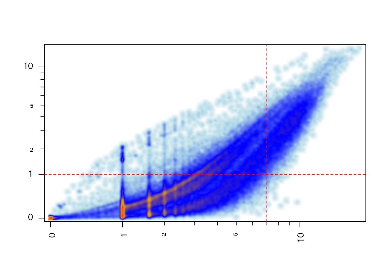
Determining reasonable cutoff values
Some of the cutoff values can be visualized by plotting the TPM versus the pseudocounts, shown below.
## For this plot, filter out all rows where TPM and abundance are zero.
if (exists("TxSE")) {
   iWhich <- (assays(TxSE[,1])[["counts"]] > 0 &
         assays(TxSE[,1])[["abundance"]] > 0);
   par("mfrow"=c(1,1), "mar"=c(5,4,4,2), "oma"=c(0,0,0,0));
   plotSmoothScatter(x=log2(1+assays(TxSE[iWhich,1])[["counts"]]),
      y=log2(1+assays(TxSE[iWhich,1])[["abundance"]]),
      xlab="counts",
      ylab="abundance",
      xaxt="n",
      yaxt="n");
   jamba::minorLogTicksAxis(1,
      logBase=2, displayBase=10, offset=1);
   jamba::minorLogTicksAxis(2,
      logBase=2, displayBase=10, offset=1);
   abline(v=log2(1+cutoffTxExpr),
      h=log2(1+cutoffTxTPMExpr),
      lty="dashed",
      col="red");
}
Salmon pseudocounts versus TPM
Another method to determine suitable cutoff values is to create an MA-plot of the data, and look for the expression below which the variability becomes very high.
Optional data normalization
Typically, RNA-seq data abundances are affected by non-experimental factors such as total mapped reads, sample quality, sequence library efficiency, etc. Despite the fact that metrics such as FPKM and TPM are intended to reduce or remove the variability between samples, there are sometimes unavoidable differences which are apparently not biological in origin.
A full description of data normalization is beyond the scope of this document, however the recommended approach to review data is to use the jamma::jammaplot() MA-plot functions, as shown above.
MA-plots of pseudocount data
The jammaplot R package is available on Github:
First show the pseudocount data:
if (exists("TxSE")) {
   if (suppressPackageStartupMessages(require(jamma))) {
      par("oma"=c(0,0,3,0));
      jamma::jammaplot(
         noiseFloor(minimum=0.0001,
            newValue=NA,
            assays(TxSE)[["counts"]]),
         transFactor=0.3,
         ylim=c(-3,3),
         ablineV=log2(1+cutoffTxExpr),
         titleBoxColor=colorjam::group2colors(colData(TxSE)$Group),
         groupSuffix="",
         titleCexFactor=1.2,
         useMean=TRUE);
      title(outer=TRUE,
         main=paste0("MA-plot using Salmon pseudocounts\n",
            paste0("Showing pseudocount cutoff value approximately ",
               log2(1+cutoffTxExpr))));
   }
}
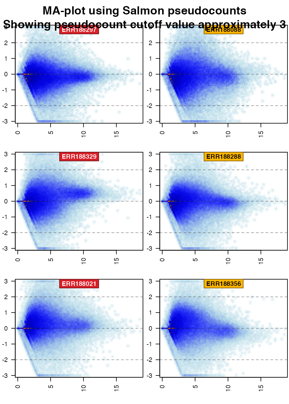
In the MA-plots above, one expects each sample to have roughly horizontal distribution, centered at y=0, which means the median transcript expression is roughly unchanged across all samples(y=0), and that the signal is roughly consistent from the low to high end of expression (horizontal).
Whenever a sample has bulk of its expression above (or below) y=0, it suggests there is overall higher (or lower) signal for all transcripts in that sample, which is counter to most assumptions of data normalization.
MA-plots of TPM data
Next show the TPM data:
if (exists("TxSE")) {
   par("oma"=c(0,0,3,0));
   jamma::jammaplot(
      noiseFloor(minimum=0.0001,
         newValue=NA,
         assays(TxSE)[["abundance"]]),
      transFactor=0.3,
      ylim=c(-3,3),
      ablineV=log2(1+cutoffTxTPMExpr),
      titleBoxColor=colorjam::group2colors(colData(TxSE)$Group),
      groupSuffix="",
      displayMAD=TRUE,
      titleCexFactor=1.2,
      useMean=TRUE);
   title(outer=TRUE,
      main=paste0("MA-plot using Salmon TPM\n",
         paste0("Showing TPM cutoff value approximately ",
            log2(1+cutoffTxTPMExpr))));
}
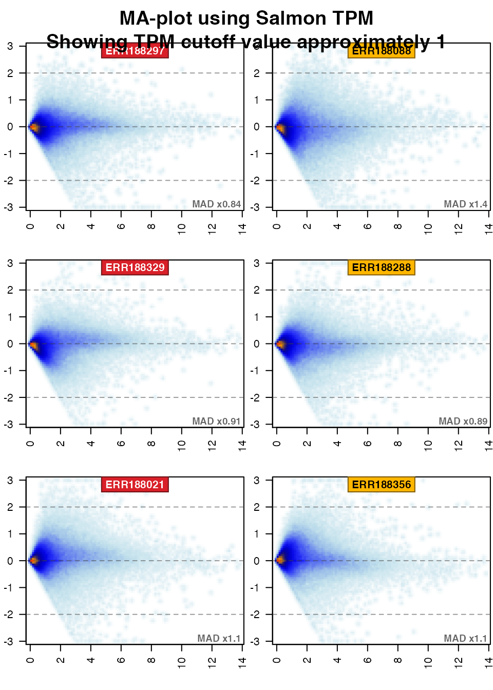
The typical remedy for certain MA-plot patterns are summarized briefly below:
- If expression is roughly horizontal for all samples, with all samples centered closely at
y=0, then no normalization is required. - If expression is roughly horizontal for all samples, with some samples centered above or below
y=0, then median normalization is recommended. - If expression is not horizontal for all samples, where some subset of samples show a slope upward, or downward from left-to-right on the MA-plot panel, the usual remedy is quantile normalization.
- If the variability above/below
y=0is substantially higher for some samples than the majority of all samples, these samples may be considered technical outliers. UsedisplayMADon thejammaplot()to view the relative variability across samples. A MAD factor threshold of 2xMAD is typically enough to identify outliers among biological replicates, or threshold 5xMAD across all samples.
Differential isoform analysis
Differential isoform analysis is carried out using the function splicejam::runDiffSplice(), which performs several convenient steps including the core function limma::diffSplice().
Design and Contrast matrices
Before statistical comparisons can be performed, the design matrix and contrast matrix must be defined. The function groups2contrasts() makes it convenient to convert group names to a set of contrasts. The group names are assumed to have underscore "_" as a delimiter between factors, for example "Wildtype_Control" and "Mutant_Treated".
if (exists("TxSE")) {
   ## Design matrix is defined by the sample groups
   iSamples <- colnames(TxSE);
   iGroups <- jamba::nameVector(
      colData(TxSE[,iSamples])$Group,
         iSamples);

   ## Use the function groups2contrasts()
   iDC <- groups2contrasts(iGroups, returnDesign=TRUE);
   iDesign <- iDC$iDesign;
   iContrasts <- iDC$iContrasts;

   printDebug("iDesign:");
   print(iDesign);
   printDebug("iContrasts:");
   print(iContrasts);

   ## Alternative method
   if (1 == 2) {
      iDesign <- stats::model.matrix(~0+iGroups);
      colnames(iDesign) <- levels(iGroups);
      rownames(iDesign) <- names(iGroups);
      # Alternative format, useful for custom contrasts
      iContrasts <- limma::makeContrasts(
         contrasts=c(
            "CA2_DE-CA2_CB",
            "CA1_DE-CA1_CB"),
         levels=iDesign);
   }
}
#> ##  (19:09:19) 09Mar2021:  iDesign:
#>           A B
#> ERR188297 1 0
#> ERR188088 0 1
#> ERR188329 1 0
#> ERR188288 0 1
#> ERR188021 1 0
#> ERR188356 0 1
#> ##  (19:09:19) 09Mar2021:  iContrasts:
#>       Contrasts
#> Levels B-A
#>      A  -1
#>      B   1
Note that it is important to keep the colnames(TxSE), design matrix, and contrast matrix in proper order. For this reason, iSamples is defined as colnames(TxSE), which should equal rownames(iDesign). Finally, colnames(iDesign) should equal rownames(iContrasts).
As a fun matrix math review, you can print the crossproduct of the design and contrast matrices to view the samples used in each contrast.
runDiffSplice()
Given an expression data matrix, design matrix, and contrast matrix, splicejam::runDiffSplice() can be called. Note that all abundance values of zero are set to NA, so they do not contribute to the analysis.
if (exists("TxSE")) {
   iMatrixTxTPM <- assays(TxSE[,iSamples])[["abundance"]];
   iMatrixTxTPM[iMatrixTxTPM == 0] <- NA;
   diffSpliceL <- runDiffSplice(
      iMatrixTx=iMatrixTxTPM,
      detectedTx=detectedTx,
      tx2geneDF=tx2geneDF,
      txColname=txColname,
      geneColname=geneColname,
      iDesign=iDesign,
      iContrasts=iContrasts,
      cutoffFDR=0.05,
      cutoffFold=1.5,
      collapseByGene=TRUE,
      spliceTest="t",
      verbose=FALSE,
      useVoom=FALSE);
   diffSpliceHitsL <- lapply(diffSpliceL$statsDFs, function(iDF){
      hitColname <- head(vigrep("^hit ", colnames(iDF)), 1);
      as.character(subset(iDF, iDF[[hitColname]] != 0)[,geneColname]);
   });
   printDebug("Differential isoform hits per contrast:");
   print(sdim(diffSpliceHitsL));
}
#> Total number of exons:  30572
#> Total number of genes:  8113
#> Number of genes with 1 exon:  0
#> Mean number of exons in a gene:  4
#> Max number of exons in a gene:  22
#> ##  (19:09:21) 09Mar2021:  Differential isoform hits per contrast:
#>     rows     class
#> B-A  644 character
Export DiffSplice results to Excel
Each contrast is summarized into two data.frame objects, representing each transcript isoform result per row, and aggregated into a per-gene summary value. For the purpose of this workflow, the per-gene summary will be saved, however the same basic steps can be applied to the per-isoform data.
PCA/BGA Clustering
Either transcript- or gene-level data may be clustered using an ordination technique such as principal components analysis (PCA) or correspondence analysis (CCA or CA).
For this workflow, between groups analysis (BGA) will be employed, as provided by the made4 Bioconductor package (Culhane et al.) In short, BGA enhances a basic ordination method by re-ordering components based upon maximal sample group separation, as opposed to maximal sample separation done by PCA. As a result, BGA is particularly effective at identifying and visualizing effects relevant to grouped experimental design, and is relatively tolerant of sources of technical noise.
Run BGA
The BGA technique is based upon results from an underlying clustering method such as PCA or COA, and therefore inherits potential weaknesses of such tools. In short, it is sometimes helpful to filter genes or transcripts by minimum expression, roughly above the level of statistical noise.
For the example below, the gene summary TPM values are used as input, and correspondence analysis (COA) is chosen as the underlying clustering algorithm.
In the absence of sample groups, BGA can be run with each biological sample in its own group. The results will be equivalent to running normal COA (or PCA).
if (exists("TxSE")) {
   if (suppressPackageStartupMessages(require(made4))) {
      bgaExprThreshold <- 5;
      bgaExprs <- assays(GeneSE)$counts;
      ## Apply a noise floor so all (data < threshold) is set to threshold
      bgaExprs[bgaExprs < bgaExprThreshold] <- bgaExprThreshold;
      ## Then require rows to have some difference between the
      ## minimum and maximum value.
      bgaExprsUse <- bgaExprs[rowMins(bgaExprs) < rowMaxs(bgaExprs),,drop=FALSE];
      #nrow(bgaExprsUse);

      geneBga <- bga(dataset=bgaExprsUse,
         classvec=nameVector(colData(GeneSE)$Group,
            colnames(GeneSE)),
         type="coa");
   }
}
BGA plotly visualization
A convenient tool to view the output in 3-D employs the plotly R package (https://CRAN.R-project.org/package=plotly ). A helper function is available splicejam::bgaPlotly3d().
At this point it is also helpful to define sample group colors which can help represent the experimental design. The function colorjam::group2colors() is used, but the main requirement is a vector of colors, where the vector names match the sample group names. If no colorSub is supplied, default colors will be defined.
Note: The steps below are disabled for the purpose of this example data, which does not contain proper sample groups with replicates. However, the commands below are adequate for a typical RNA-seq experimental design.
if (1 == 2 &&
      suppressPackageStartupMessages(require(made4)) &&
      suppressPackageStartupMessages(require(plotly))) {
   colorSubBga <- colorjam::group2colors(colData(GeneSE)$Group);

   geneBgaly <- bgaPlotly3d(geneBga,
      axes=c(1,2,3),
      colorSub=colorSubBga,
      useScaledCoords=FALSE,
      drawVectors="none",
      drawSampleLabels=FALSE,
      superGroups=gsub("_.+", "", geneBga$fac),
      ellipseType="none",
      sceneX=0, sceneY=1, sceneZ=1,
      verbose=TRUE);
   print(geneBgaly);

   ## Example for saving the BGA plot to an HTML file
   #
   #htmlwidgets::saveWidget(geneBgaly,
   #   file="RNAseq_BGA_clustering.html",
   #   title="RNA-seq BGA clustering");
}