Create a Sashimi Plot
James M. Ward
2026-07-27
Source:vignettes/create-a-sashimi-plot.Rmd
create-a-sashimi-plot.RmdOverview
This vignette is intended to describe how to create a Sashimi plot using RNA-seq data.
Outline
-
sashimiDataConstants(): Prepare data inside anenvironmentwhich is used to prepare figures. -
splicejamFigure(): The core function to produce a Splicejam sashimi plot figure.
Alternatively, open an R-shiny app:
Requirements
There are three basic requirements for a Sashimi plot:
-
Gene-exon structure: The easiest input is a GTF
.gtfor GFF3.gfffile. -
RNA-seq coverage data: Typically bigwig
.bwfiles. -
Splice junction data: Typically BED12
.bed, bigBed.bb, or STAR'SJ.out.tab'formatted file.
Each type of data will be described below.
Gene-exon structure
There are several sources of gene-exon structures:
GTF File
GTF or GFF file, for example Gencode GTF (https://www.gencodegenes.com).
A GTF file is sufficient to cover all gene-transcript-exon requirements for Splicejam.
When a GTF file and corresponding transcripts are used for STAR alignment, and/or Salmon/Kallisto quantitation, we recommend using the same file as input to Splicejam.
-
The GTF should have the following fields defined:
- ‘gene_name’:
charactergene symbol. Its values will be used to represent genes in thedata.framereferred to as'tx2geneDF'. - ‘transcript_id’:
charactertranscript identifier, for example'ENST0000001.2'. Its values will be used in'tx2geneDF'in column ‘transcript_id’. - Note the ‘gene_id’ column is not typically used as the primary key for genes.
- ‘gene_name’:
How the GTF file is used:
- The GTF or GFF file is used to prepare
'tx2geneDF'which associates transcripts'transcript_id'to genes'gene_name', usingmakeTx2geneFromGtf(). It also parses other GTF entries in column 9 (annotations), to include in the resultingtx2geneDFoutputdata.frame. - The GTF or GFF file is converted to
TxDbannotation database usingtxdbmaker::makeTxDbFromGFF(). ThisTxDbis saved in a local file with extension'.txdb'for re-use if needed. - The
TxDbdata is used to produceexonsByTx, and if the ‘CDS’ field is defined in the GTF file it also producescdsByTx. The CDS is used to distinguish non-coding exons (thin exons) from coding exons (wide exons) in the Splicejam sashimi plot.
TxDb and tx2geneDF
A TxDb is typically produced using the Bioconductor
package ‘txdbmaker’, see txdbmaker::makeTxDb() for various
types of input.
-
Note that
TxDbinput is not sufficient alone, since Splicejam requires ‘gene_name’ to be associated with ‘transcript_id’.- Bioconductor provides several Txdb data packages (see BiocView https://bioconductor.org/packages/release/BiocViews.html#___TxDb).
For example, to install the package for hg19 UCSC knownGenes TxDb,
BiocManager::install("TxDb.Hsapiens.UCSC.hg19.knownGene"). - The TxDb specification includes ‘gene_id’ but not ‘gene_name’,
instead it must be provided, or produced using Bioconductor organism
annotation data, for example the Human annotation package is called
'org.Hs.eg.db'. - Most Bioconductor packages define ‘gene_id’ using ENTREZID, however
it is not clearly documented. For example
TxDb.Hsapiens.UCSC.hg38.knownGenedoes not indicate that is uses ENTREZID, which is surprising because UCSC knownGene typically uses its own gene identifiers to enable them to provide gene loci which are not represented in the NCBI Gene release. Nonetheless, one can convert UCSC knownGene in hg38 usingorg.Hs.eg.db::org.Hs.egSYMBOLusing something like this:AnnotationDbi::mget("1", org.Hs.eg.db::org.Hs.egSYMBOL).
- Bioconductor provides several Txdb data packages (see BiocView https://bioconductor.org/packages/release/BiocViews.html#___TxDb).
For example, to install the package for hg19 UCSC knownGenes TxDb,
Methods to produce
'tx2geneDF'are described intximport::tximport(), which also includes references to other resources. One straightforward approach is to use a GTF or GFF file withmakeTx2geneFromGtf().
GRangesList objects, and tx2geneDF
GRangesList objects ‘exonsByTx’, ‘exonsByGene’, and
‘cdsByTx’ may be provided, for example by using
GenomicFeatures::exonsBy() and
GenomicFeatures::cdsBy() or equivalent.
These objects are used to produce flattened exon models, for example
a flat exon model for transcript would combine exonsByTx
with cdsByTx to represent non-coding and coding regions as
narrow and wide exons, respectively. The output is
flatExonsByTx.
Alternatively, flatExonsByTx can be provided directly,
for example it can be prepared using flattenExonsBy().
The flatExonsByTx is used together with
tx2geneDF to prepare flatExonsByGene.
Alternatively, it may be prepared upfront for example using
flattenExonsBy().
Note that gene exons are numbered based upon the observed exon structure of the transcripts provided. Therefore, when using
detectedTxto define a subset of detected transcripts, the exon numbers may differ from the output if using all annotated transcripts. This distinction was intentional, and motivated by numerous Gencode comprehensive transcripts which may not be observed in practice. However, one may prepare flattened exons using all transcripts to override this decision.
- The
tx2geneDFshould be adata.framewith minimal columns ‘transcript_id’ and ‘gene_name’. These data associate transcripts to genes. -
exonsByTxshould be named by ‘transcript_id’ as intx2geneDF. -
cdsByTxshould be named by ‘transcript_id’ as intx2geneDF. It is optional, and when provided it is used to produce narrow and wide exons in the resulting gene-transcript-exon model.
Use of detected transcripts
The recommended workflow is to use an appropriate set of “detected transcripts” with Splicejam. The motivation is to represent observed exon structure, which is beneficial when used together with Gencode comprehensive transcript data. The comprehensive data often includes numerous extraneous transcripts which may make it difficult to interpret isoform changes in the given experiment.
Instead, using “detected transcripts” is helpful to review scenarios where, for example, isoform A switches to isoform B. There may be 12 other potential isoforms without supporting data, and they would not be helpful to assess the A-to-B isoform switch.
Note that transcript quantitation is usually necessary to define detected transcripts, for example using Salmon or Kallisto.
Splicejam provides splicejam::defineDetectedTx() with
heuristics to help define detected transcripts, typically using some
combination of minimum counts, minimum estimated TPM abundance, and
minimum percent max of each. It typically reduces the total transcripts
by about 60% the original size, the vast majority of transcripts removed
have zero or near-zero quantitative values.
We found it beneficial to apply:
- Minimum count, to require some minimum plausible supporting data.
- Minimum TPM abundance, to require some minimum fractional transcript versus the overall observed transcriptome.
- Percent max per gene, to require a minor isoform to comprise at least 10% of the highest group mean within the same sample group. This option uses ‘TPM’ by default, so the evaluation is done at ‘molar’-like level and is relatively independent of transcript length. This filter helps remove extremely low abundance transcripts from extremely high abundance genes, for example GAPDH and ACTB may have 20 copies of an obscure isoform, compared with over 120,000 counts of the predominant isoform. The 20 copies may be biologically real, but in our experience has not typically represented signal useful to downstream analysis and visualization.
For additional information about transcript quantitation, see:
Salmon (Patro et al 2017, https://combine-lab.github.io/salmon/)
Kallisto (Bray et al 2016, https://pachterlab.github.io/kallisto/about)
TxDb Bioconductor package
This example uses Bioconductor data package
TxDb.Mmusculus.UCSC.mm10.knownGene which represents UCSC
known genes for the mouse mm10 genome assembly.
First we assemble all exons by transcript, then all CDS exons by transcript. We will use these exons to assemble annotated gene models.
options("warn"=-1);
suppressPackageStartupMessages(library(splicejam));
suppressPackageStartupMessages(library(jamba));
suppressPackageStartupMessages(library(kableExtra));
if (suppressPackageStartupMessages(require(TxDb.Mmusculus.UCSC.mm10.knownGene))) {

   # First obtain exons by transcript
   exonsByTxMm10 <- exonsBy(TxDb.Mmusculus.UCSC.mm10.knownGene,
      by="tx",
      use.names=TRUE);
   values(exonsByTxMm10@unlistData)$feature_type <- "exon";
   values(exonsByTxMm10@unlistData)$subclass <- "exon";

   # For added insight, obtain CDS exons by transcript (optional)
   cdsByTxMm10 <- cdsBy(TxDb.Mmusculus.UCSC.mm10.knownGene,
      by="tx",
      use.names=TRUE);
   values(cdsByTxMm10@unlistData)$feature_type <- "cds";
   values(cdsByTxMm10@unlistData)$subclass <- "cds";
}
The TxDb objects do not permit storing gene symbols, so
the example uses the Bioconductor annotation package
org.Mm.eg.db to assign gene_name values. For
values not found in org.Mm.eg.db, we use the format
LOC# to indicate the Entrez gene ID, for example Entrez
gene ID 1234 would be represented LOC1234.
if (require(TxDb.Mmusculus.UCSC.mm10.knownGene)) {

   # Now prepare tx_name, gene_id, gene_name data.frame,
   # surprisingly difficult
   tx2geneMm10 <- suppressMessages(
      AnnotationDbi::select(TxDb.Mmusculus.UCSC.mm10.knownGene,
         keys(TxDb.Mmusculus.UCSC.mm10.knownGene, "GENEID"),
         columns=c("GENEID","TXNAME"),
         keytype="GENEID"
      )
   );
   tx2geneMm10 <- renameColumn(tx2geneMm10,
      from=c("GENEID", "TXNAME", "TXTYPE"),
      to=c("gene_id", "transcript_id", "transcript_type"));

   # add gene_name using org.Mm.eg.db
   if (suppressPackageStartupMessages(require(org.Mm.eg.db))) {
      gene_ids <- values(genes(TxDb.Mmusculus.UCSC.mm10.knownGene))$gene_id;
      gene_namesL <- mget(gene_ids,
         org.Mm.egSYMBOL,
         ifnotfound=NA);
      ## Convert list to vector taking the first gene_name each
      ## (All genes should only have one SYMBOL but there is no
      ## hard constraint so we should make absolutely sure to
      ## use only one value per gene.)
      gene_names <- unlist(heads(S4Vectors::List(gene_namesL), 1));
      ## Replace NA with LOC# format
      ## Note we use gsub() to ensure the data fits the expected format
      if (any(is.na(gene_names))) {
         gene_na <- which(is.na(gene_names));
         gene_names[gene_na] <- gsub("^([0-9]+)$", "LOC\\1",
            names(gene_names[gene_na]));
      }
      tx2geneMm10$gene_name <- gene_names[as.character(tx2geneMm10$gene_id)];
   } else {
      ## If we have no gene annotations, use the gene_id values
      tx2geneMm10$gene_name <- as.character(tx2geneMm10$gene_id);
   }
   # print the first 20 rows to show the content
   print(head(tx2geneMm10, 20));
}
#> Loading required package: TxDb.Mmusculus.UCSC.mm10.knownGene
Next we flatten transcript exons to the gene level using the function
splicejam::flattenExonsBy().
We also flatten exons to the transcript level, which has the effect of combining CDS exons alongside non-CDS exons. The result is used when plotting transcript exon structures.
In both cases, the argument genes=c("Gria1", "Ntrk2") is
used as a convenience to produce data for only these two genes.
We recommend using detected transcripts here, with the argument
detectedTx.
if (require(TxDb.Mmusculus.UCSC.mm10.knownGene)) {
   # flatten exons to the gene level
   # for speed, we will only process "Gria1", and "Ntrk2"
   flatExonsByGeneMm10 <- flattenExonsBy(exonsByTx=exonsByTxMm10,
      cdsByTx=cdsByTxMm10,
      by="gene",
      genes=c("Gria1", "Ntrk2"),
      tx2geneDF=tx2geneMm10,
      verbose=FALSE);

   # to be fancy, also flatten transcripts, to include CDS ranges
   flatExonsByTxMm10 <- flattenExonsBy(exonsByTx=exonsByTxMm10,
      cdsByTx=cdsByTxMm10,
      tx2geneDF=tx2geneMm10,
      by="tx",
      genes=c("Gria1", "Ntrk2"));
}
#> Loading required package: TxDb.Mmusculus.UCSC.mm10.knownGene
Plot gene-exon models using gene2gg()
Once the gene-transcript-exon data is prepared, the exon structure
can be plotted using the function splicejam::gene2gg():
if (require(TxDb.Mmusculus.UCSC.mm10.knownGene)) {
   # Pull out Gria1
   grlGria1 <- flatExonsByGeneMm10[["Gria1"]];

   ## Plot a basic gene-exon structure
   ggGria1exons <- gene2gg(gene="Gria1",
      flatExonsByGene=flatExonsByGeneMm10,
      exonLabelSize=6);
   print(ggGria1exons + ggtitle("Gria1 exons"));

   ## Compare to the gene structure without compressing introns
   gg1full <- gene2gg(gene="Gria1",
      flatExonsByGene=flatExonsByGeneMm10,
      compressGaps=FALSE)
   print(gg1full);

   ## Plot a slightly more detailed gene-transcript-exon structure
   ggGria1exonsTx <- gene2gg(gene="Gria1",
      flatExonsByGene=flatExonsByGeneMm10,
      flatExonsByTx=flatExonsByTxMm10,
      tx2geneDF=tx2geneMm10);
   print(ggGria1exonsTx + ggtitle("Gria1 (compressed introns)"));

   ## Notice how difficult it is to see exon15 and exon16 are
   ## mutually exclusive exons
   gg2full <- gene2gg(gene="Gria1",
      flatExonsByGene=flatExonsByGeneMm10,
      flatExonsByTx=flatExonsByTxMm10,
      tx2geneDF=tx2geneMm10,
      compressGaps=FALSE);
   print(gg2full + ggtitle("Gria1 (uncompressed introns)"));

}
#> Loading required package: TxDb.Mmusculus.UCSC.mm10.knownGene
Coverage and Junctions data
All coverage data, and junction data, should be described in a
data.frame 'filesDF'. It should have the
following columns:
‘sample_id’: Sample identifier, and in reality it should represent sample groups even when multiple replicates are available for each group. All files associated with each ‘sample_id’ are combined in strand-specific manner.
‘url’: A web URL https link, or path to a local file, or the
charactername of columnvalues()when supplying coverage asGRangesobject'covGR'.-
‘type’:
characterstring, one of:- ‘bw’: bigwig coverage file
- ‘junction’: BED12, bigBed (using bed12), or
'SJ.out.tab'file produced by STAR. - ‘coverage_gr’: coverage provided as
GRangesas'covGR'. The names invalues()must match the character string in ‘url’ for this row.
‘scale_factor’: optional
numericscalar used to adjust the magnitude of signal, applied by multiplying the scale factor by the score. The scale factor is intended to provide a method to normalize data without creating a new coverage or junction file.
Coverage data
The recommended input for coverage data is via bigWig
'.bw' or '.bigwig' files. BigWig data are
imported using the amazing package
cpp11bigwig::read_bigwig().
The bigwig files can be stored on the local file system, or remote via https web URL. Local access is faster, but remote access is fairly close due to ‘cpp11bigwig’, and using memoise cache removes the distinction after each gene is loaded at least once.
It is possible to provide coverage as GRanges data with
columns storing the coverage as NumericList, or other
object coercible to list. The GRanges entries
must exactly match the names() of the corresponding
flatExonsByGene, for example 'Gria1_exon1',
'Gria1_exon2a', 'Gria1_exon2b', etc. The
colnames of values() should exactly match the
'sample_id' column values in the filesDF
data.frame.
Note that coverage in either case should only represent one strand, therefore samples are expected to have “+” and “-” strand coverage data.
Use the ‘farrisdata’ package, Github
'jmw86069/farrisdata', for an example of filesDF:
filesDF <- farrisdata::farris_sashimi_files_df;
jamba::kable_coloring(jamba::mixedSortDF(filesDF, byCols=c(1, 3)),
   row.names=FALSE,
   row_color_by="sample_id",
colorSub=farrisdata::colorSub)Coverage in GRanges format
The GRanges object below uses an example set of exons,
test_exon_wide_gr, and corresponding coverage
GRanges is test_exon_wide_gr. Note that both
share the same names and genomic coordinates.
There is no coverage defined for introns.
data(test_exon_wide_gr);
test_exon_wide_gr;
#> Loading required namespace: GenomicRanges
#> GRanges object with 4 ranges and 1 metadata column:
#>         seqnames      ranges strand |   gene_name
#>            <Rle>   <IRanges>  <Rle> | <character>
#>   wide1     chr1     100-200      + |   TestGene1
#>   wide2     chr1 10300-10400      + |   TestGene1
#>   wide3     chr1 20500-20750      + |   TestGene1
#>   wide4     chr1 39900-40000      + |   TestGene1
#>   -------
#>   seqinfo: 1 sequence from an unspecified genome; no seqlengths
data(test_cov_wide_gr);
test_cov_wide_gr;
#> GRanges object with 4 ranges and 1 metadata column:
#>         seqnames      ranges strand |        sample_A
#>            <Rle>   <IRanges>  <Rle> |   <NumericList>
#>   wide1     chr1     100-200      + | 246,248,261,...
#>   wide2     chr1 10300-10400      + | 195,202,198,...
#>   wide3     chr1 20500-20750      + | 195,189,178,...
#>   wide4     chr1 39900-40000      + | 260,257,253,...
#>   -------
#>   seqinfo: 1 sequence from an unspecified genome; no seqlengths
Junctions data
Splice junction data are provided as a link to local file, or remote web https URL. Entries can be in BED6 format, BED12 format, or ‘SJ.out.tab’ format produced by STAR.
For BED formats, data is accepted as BED or bigBed, although the bigBed format is substantially faster.
Splice junction data can be provided in two forms:
- Files in
BED6orBED12format, accessible either as a file or web URL. TheBED6format uses the score column to count reads, and uses the genomic coordinates to indicate the splice junction span. - The
BED12format is inverted, so there is one base on each side, and the junction is in the middle. In this case, the one base is trimmed from each side, and the internal region is used to indicate the junction. This approach works best when the overhang is fixed at 1 base on each side.
For more insight into creating a Sashimi plot manually, see the help
for data splicejam::test_junc_wide_gr.
Splicejam Data Environment
With the necessary data available, you create a Splicejam
environment to contain the data.
sjenv <- sashimiDataConstants(...)
By default, if you provide no supporting data, the default argument
empty_uses_farrisdata=TRUE means it will prepare supporting
data for the Farris et al 2019 publication.
However, a small subset of data are available with the test data
sjenvtest.
The two most common types of input are:
- GTF file.
- TxDb file, and tx2geneDF
data.frame.
For example, the typical pattern:
sjenv <- new.env();
sjenv <- sashimiDataConstants(envir=sjenv,
   empty_uses_farrisdata=FALSE,
   filesDF=filesDF,
   gtf=gtf);
You can use jamba::sdim() to describe the data. In this
case, we will use sjenvtest as the
environment:
data(sjenvtest)
jamba::sdim(sjenvtest)
#>                 rows cols                 class
#> color_sub         16                  character
#> default_gene       1                  character
#> filesDF           12    6            data.frame
#> flatExonsByGene    2      CompressedGRangesList
#> flatExonsByTx     10      CompressedGRangesList
#> tx2geneDF         10    7            data.frame
Splicejam Figure
The core function splicejamFigure() prepares the
multi-panel plot for a given gene.
To see progress, enable it with
progressr::handlers(global=TRUE).
# optionally enable progress bar
# progressr::handlers(global=TRUE)

data(sjenvtest)
sjfig <- splicejamFigure(sjenv=sjenvtest,
   gene="Gria1")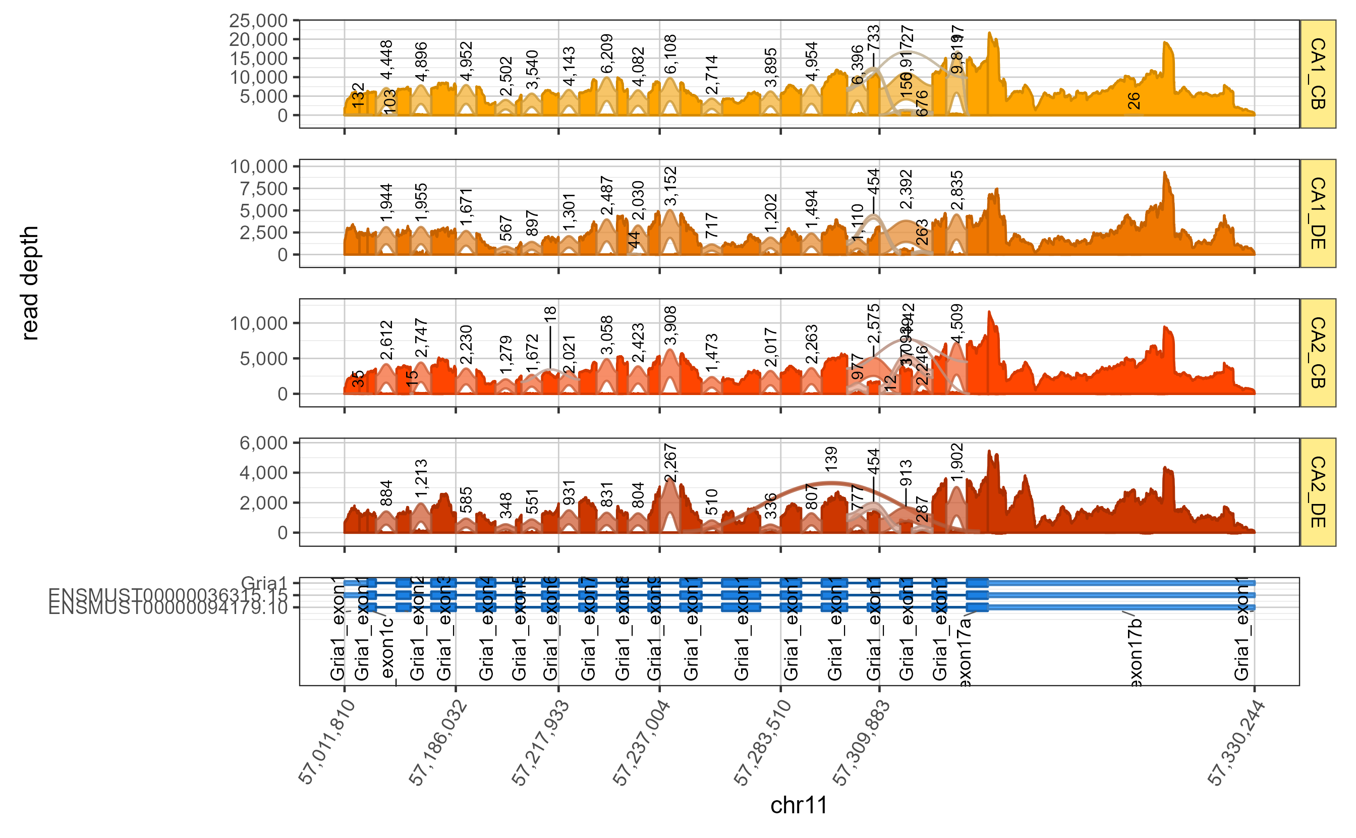
It does not enable memoise by default, however it is strongly recommended.
data(sjenvtest)
# Enable memoise
sjfig <- splicejamFigure(sjenv=sjenvtest,
   use_memoise=TRUE,
   gene="Gria1")
Note that splicejamFigure() does the work of calling
prepareSashimi(), plotSashimi(),
gene2gg(), then assembles the panels using
patchwork by default. Various customizations can be passed
via ‘…’ especially with plotSashimi() arguments.
Zoom into specific exons
The splicejamFigure() arguments include two methods to
zoom to specific exons.
- ‘exon_range’:
charactervector with two exons, for example:use_exon_range=c('Gria1_exon13', 'Gria1_exon16') - ‘display_coords’:
integervector with start and end positions. Note the coordinates must be valid for the gene being displayed.
data(sjenvtest)
sjfig_zoom <- splicejamFigure(sjenv=sjenvtest,
   use_exon_range=c('Gria1_exon13', 'Gria1_exon16'),
   use_memoise=TRUE,
   gene="Gria1")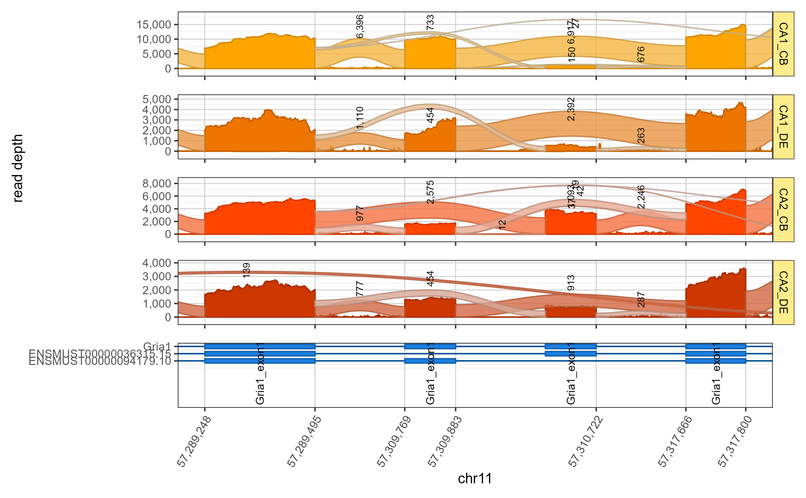
Adjust layout
You can adjust the layout, for example to impose two columns use
layout_ncol=2
data(sjenvtest)
sjfig_zoom_2col <- splicejamFigure(sjenv=sjenvtest,
   use_exon_range=c('Gria1_exon13', 'Gria1_exon16'),
   layout_ncol=2,
   use_memoise=TRUE,
   gene="Gria1")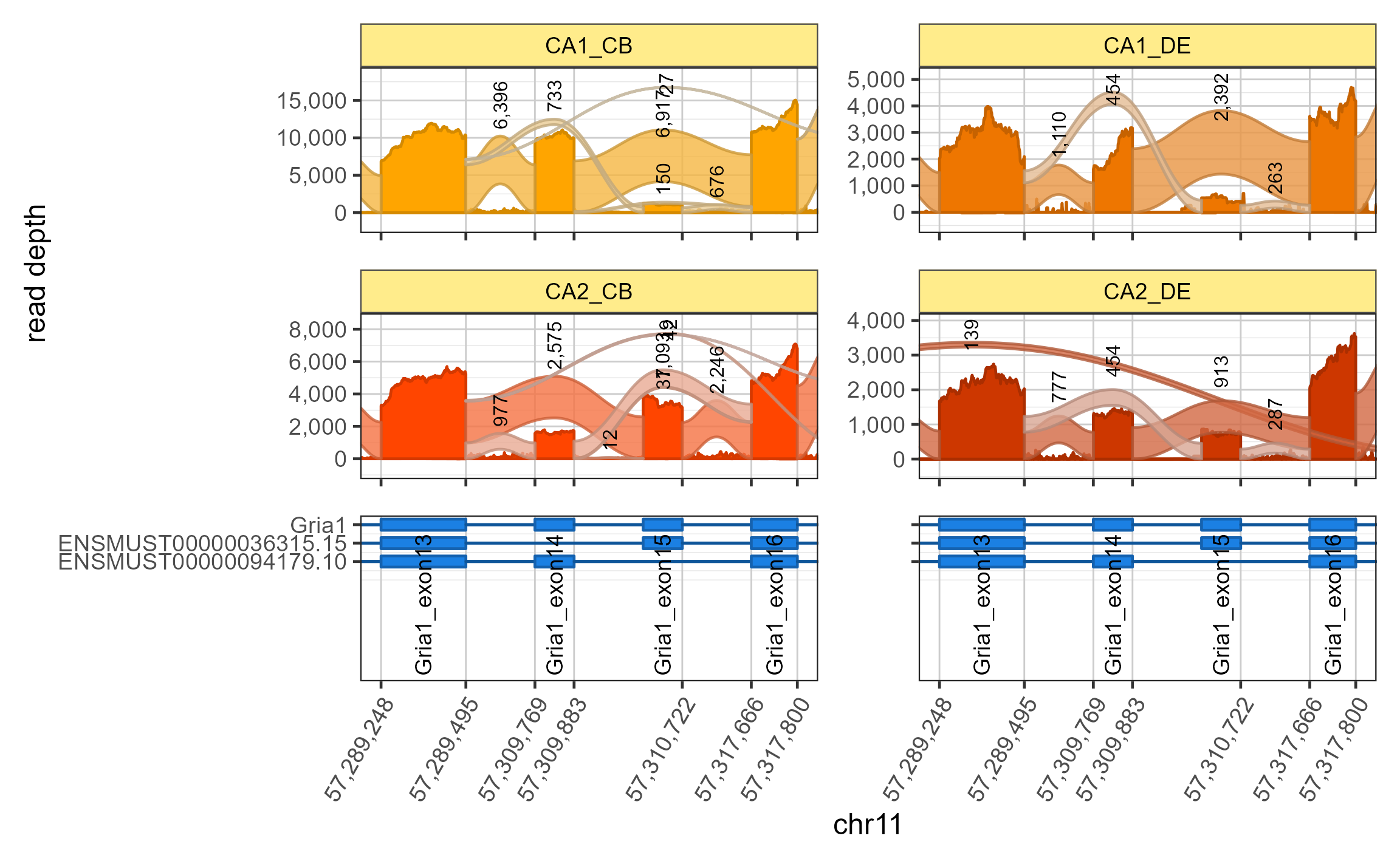
Splicejam Shiny App
When the sjenv data environment is
prepared, you can run the Splicejam shiny app:
data(sjenvtest)
launchSashimiApp(envir=sjenvtest)
Start the Shiny app on a different port
Two common options to customize are ‘host’ and ‘port’. By using host=‘0.0.0.0’ it makes the Sashimi app accessible to other computers, provided they can see your computer IP address.
Note that in general, the only computers that are able to see your computer IP address are those on the same network as your computer. That goes for company or school intranet, or within your home network.
A custom ‘port’ makes it easier to use a consistent port number,
otherwise it is more or less random. On most computers, it requires some
administrative permission to use a port lower than 8000, so a common
recommendation is port='8080' or something easy to
remember.
launchSashimiApp(
   empty_uses_farrisdata=FALSE,
   envir=sjenv,
   options=list(
      port=8080,
      host="0.0.0.0"))
Custom options
Several elements in the Splicejam app can be set as defaults.
-
default_gene:
charactergene symbol for the initial figure. - layout_ncol: default number of columns for the panel layout.
- panel_height: height for each panel in pixels, default 200.
- gene_panel_height: height for the gene panel, default is 400.
-
min_junction_reads:
numericminimum junction reads. -
share_y_axis:
logicalwhether to use shared (fixed) y-axis range across all panels, default FALSE. -
use_exon_range:
charactervector with first and last exon to include by default. -
gene_coords_default: initial
integercoordinate range, default NULL shows the whole gene. -
label_junctions:
logicalwhether to display junction counts, default TRUE. -
show_gene_model:
logicalwhether to show the gene-exon model, default TRUE. -
font_sizing:
characterlabel matching one of the options shown, default is “Default”. Other options range from “-4 smaller” to “+4 larger”. -
exon_font_sizing:
characterlabel matching one of the options shown, default is “Default”. See comment for font_sizing. -
junction_alpha:
numericdefault alpha transparency, default 0.7 is 70% opaque. -
junction_arc_factor:
characterstring matching one of the options shown, default is “Default”. Options range from “-2 flat” to “+3 higher”. -
junction_arc_minimum:
numericminimum arc height per junction, default 500 ensures the arc is at least 500 y-axis units high. -
aboutExtra:
characterorhtmlwidgetsformatted tags suitable to display as HTML, shown in the “About” tab to describe the data being displayed. It is normally defined insidesashimiAppConstants().
For example:
data(sjenvtest)
# or prepare your own environment
# sjenv <- sashimiDataConstants()

sjenvtest$default_gene <- "Ntrk3"
sjenvtest$panel_height <- 150;
sjenvtest$gene_panel_height <- 300;
sjenvtest$use_exon_range <- c("Ntrk3_exon1", "Ntrk3_exon23a");

launchSashimiApp(envir=sjenvtest)