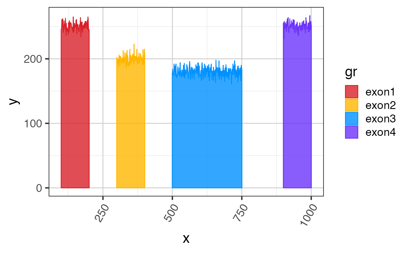
Convert exon coverage to polygons

Usage

exoncov2polygon(
  gr,
  covNames = NULL,
  sample_id = NULL,
  baseline = NULL,
  gapWidth = getOption("splicejam.gap", 250),
  doPlot = FALSE,
  coord_style = c("fortify", "base", "list", "all"),
  ref2c = NULL,
  compress_introns = TRUE,
  doSimplify = TRUE,
  verbose = FALSE,
  ...
)

Arguments

gr: GRanges where colnames(GenomicRanges::values(gr)) is present in covNames, and contains data with class NumericList.
covNames: character vector contained in colnames(GenomicRanges::values(gr)).
baseline: numeric vector of length 0, 1 or length(gr). If baseline has names matching names(gr) they will be used for each gr entry; if baseline is not named, it is extended to length(gr). The baseline value is added to the coverage for each exon to offset the polygon as needed.
gapWidth: integer value, default 200 from options('splicejam.gap'), passed to make_ref2compressed() to set a fixed with for gap, thus compressing introns to a fixed visual size. When NULL, it uses 3.3 times the median feature length.
coord_style: character value to define the output style: "base" returns a matrix with polygons separated by a row of NA values; "fortify" returns a data.frame intended for ggplot2, with columns "cov" and "gr" indicating the values in covNames and names(gr) used to separate each polygon.
ref2c: optional list containing output from make_ref2compressed(), used to compress the GRanges coordinates.
compress_introns: logical indicating whether to compress the coverage polygon coordinates to approximately the same number of pixels per inch as the exon polygons. This option greatly reduces the size of the polygon, since introns are already about 50 to 100 times wider than exons, and when ref2c is supplied, the introns are visibly compressed to a fixed width on the x-axis. The data has many more x-axis coordinates than the data visualization, this argument is intended to reduce the intron coordinates accordingly.
verbose: logical indicating whether to print verbose output.
...: additional arguments are ignored.

Value

output dependent upon coord_style:

"fortify" returns data.frame in tall format, sufficient to use with ggplot2 functions. Each polygon is separated by rows where x,y values are NA.
"list" returns a list with numeric matrix objects.
"base" returns a list with numeric matrix objects, each of which contains NA as the last coordinate, so that each matrix can be rbind() and used for vectorized plotting.
"all" returns a list with all the data formats.

Details

This function is a workhorse function that converts a GRanges object containing column values with NumericList coverage data, into a full data.frame sufficient to define ggplot2 and other coverage polygon plots.

An interesting argument is baseline which allows each exon in the gr GRanges object to be offset from zero, in order to make certain features visually easier to distinguish.

This function also calls simplifyXY() which reduces the stored polygon detail for regions whose coordinates are compressed on the x-axis, taking roughly the max value for each point.

The default output is roughly similar to broom::tidy() in that it converts a custom R object into a tidy data.frame suitable for use by ggplot2 and other tidy workflows.

The function getGRcoverageFromBw() takes a set of bigWig files and returns a GRanges object whose columns contain NumericList data, which is the intended input for exoncov2polygon().

Examples

# use some test data
suppressPackageStartupMessages(library(GenomicRanges));
suppressPackageStartupMessages(library(ggplot2));

data(test_cov_gr);
# prepare polygon coordinates
exondf <- exoncov2polygon(test_cov_gr, covNames="sample_A");

# for testing, make bigger introns
toadd <- c(0, 4000, 8000, 16000) + rep(c(0, 20000, 40000, 60000), each=4)
test_cov_gr2 <- GenomicRanges::GRanges(
   seqnames=rep(seqnames(test_cov_gr), length.out=length(toadd)),
   ranges=IRanges::IRanges(start=start(test_cov_gr) + toadd, end=end(test_cov_gr) + toadd))
names(test_cov_gr2) <- paste0("exon", jamba::padInteger(seq_along(toadd)))
GenomicRanges::values(test_cov_gr2)$sample_A <- GenomicRanges::values(test_cov_gr)$sample_A;

# for testing, add gap coverage
test_cov_gr_gaps <- getGRgaps(test_cov_gr2);
names(test_cov_gr_gaps) <- paste0("intron", jamba::padInteger(seq_along(test_cov_gr_gaps)));
GenomicRanges::values(test_cov_gr_gaps)$sample_A <- IRanges::NumericList(
   lapply(width(test_cov_gr_gaps), function(n){sample(1:15, replace=TRUE, size=n)}))
test_cov_gr2 <- sort(c(test_cov_gr2, test_cov_gr_gaps))
# for testing, add more "samples"
GenomicRanges::values(test_cov_gr2)$sample_B <- GenomicRanges::values(test_cov_gr2)$sample_A;
GenomicRanges::values(test_cov_gr2)$sample_C <- GenomicRanges::values(test_cov_gr2)$sample_A;

# ref2c
ref2c <- make_ref2compressed(gr=test_cov_gr2[grep("exon", names(test_cov_gr2))])

exondf2a <- exoncov2polygon(test_cov_gr2, covNames=c("sample_A", "sample_B", "sample_C"))
exondf2 <- exoncov2polygon(test_cov_gr2, covNames=c("sample_A", "sample_B", "sample_C"), ref2c=ref2c)

# create a ggplot
gg3 <- ggplot2::ggplot(exondf2,
      ggplot2::aes(x=x, y=y, group=gr, fill=gr, color=gr)) +
   ggforce::geom_shape(alpha=0.8, stat="unpack_polygon") +
   colorjam::theme_jam() +
   ggplot2::facet_wrap(~cov, ncol=1) +
   ggplot2::scale_x_continuous(trans=ref2c$trans_grc) +
   colorjam::scale_fill_jam() +
   colorjam::scale_color_jam();
print(gg3);