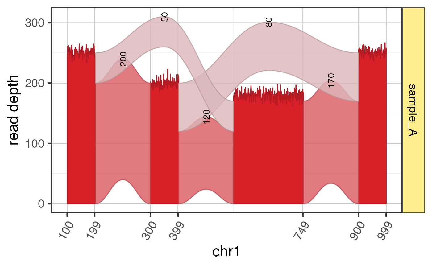
Jam Sashimi plot

Jam Sashimi plot

plotSashimi(
  sashimi,
  show = c("coverage", "junction", "junctionLabels"),
  coord_method = c("scale", "coord", "none"),
  exonsGrl = NULL,
  junc_color = alpha2col("goldenrod2", 0.3),
  junc_fill = alpha2col("goldenrod2", 0.9),
  junc_alpha = 0.8,
  junc_accuracy = 1,
  fill_scheme = c("sample_id", "exon"),
  color_sub = NULL,
  ylabel = "read depth",
  xlabel = NULL,
  xlabel_ref = TRUE,
  use_jam_themes = TRUE,
  apply_facet = TRUE,
  facet_scales = "free_y",
  ref2c = NULL,
  label_coords = NULL,
  do_highlight = FALSE,
  verbose = FALSE,
  ...
)

Arguments

sashimi	Sashimi data prepared by prepareSashimi() which is a list with covDF coverage data in data.frame format, juncDF junction data in data.frame format, juncLabelDF junction label coordinates in data.frame format, exonLabelDF exon label coordinates per coverage polygon in data.frame format, ref2c list output from make_ref2compressed() to transform genomic coordinates.
show	character vector of Sashimi plot features to include: "coverage" sequence read coverage data; "junction" splice junction read data.
coord_method	character value indicating the type of coordinate scaling to use: "scale" uses ggplot2::scale_x_continuous(); "coord" uses ggplot2::coord_trans(); "none" does not compress genomic coordinates.
exonsGrl	GRangesList object with one or more gene or transcript exon models, where exons are disjoint (not overlapping.)
junc_color, junc_fill	character string with valid R color, used for junction outline, and fill, for the junction arc polygon. Alpha transparency is recommended for junc_fill so overlapping junction arcs are visible.
junc_alpha	numeric value between 0 and 1, to define the alpha transparency used for junction colors, where 0 is fully transparent, and 1 is completely non-transparent.
fill_scheme	character string for how the exon coverages will be color-filled: "exon" will define colors for each distinct exon, using the GRanges names from flatExonsByGene; "sample_id" to color all exons the same by sample_id.
color_sub	optional character vector of R compatible colors or hex strings, whose names are used to color or fill features in the ggplot object. For example, if fill_sheme="sample_id" the color_sub should have names for each "sample_id" value. If any values are missing, they will be filled in using colorjam::rainbowJam().
ylabel	character string used as the y-axis label, by default "score" reflects the coverage score and junction score, respectively for coverage and junction data. Scores are also adjusted using the scale_factor value for each sample_id as defined in the filesDF. Set to NULL to hide the y-axis label completely.
xlabel	character string used to define the x-axis name, which takes priority over argument xlabel_ref. When xlabel is NULL and xlabel_ref is FALSE, then the x-axis name is "", which displays no x-axis label.
xlabel_ref	logical indicating whether the x-axis name should be determined by the reference (chromosome).
use_jam_themes	logical indicating whether to apply colorjam::theme_jam(), by default for the ggplot theme.
apply_facet	logical indicating whether to apply ggplot2::facet_wrap() with "~sample_id" defining each panel.
facet_scales	character value used as "scales" argument in ggplot2::facet_wrap() when apply_facet=TRUE.
ref2c	optional output from make_ref2compressed() used to compress axis coordinates during junction arc calculations.
label_coords	numeric vector length 2, optional range of genomic coordinates to restrict labels, so labels are not arranged by ggrepel::geom_text_repel() even when coord_cartesian() is used to zoom into a specific x-axis range.
verbose	logical indicating whether to print verbose output.
...	additional arguments are sent to grl2df().

Details

This function uses Sashimi data prepared by prepareSashimi() and creates a ggplot graphical object ready for visualization. As a result, this function provides several arguments to customize the visualization.

See also

Other jam plot functions: bgaPlotly3d(), factor2label(), gene2gg(), grl2df(), jitter_norm(), prepareSashimi(), stackJunctions()

Other jam ggplot2 functions: gene2gg(), geom_diagonal_wide_arc(), splicejam-extensions, to_basic.GeomShape()

Other splicejam core functions: exoncov2polygon(), gene2gg(), grl2df(), make_ref2compressed(), prepareSashimi()

Examples

suppressPackageStartupMessages(library(GenomicRanges));
data(test_exon_gr);
data(test_junc_gr);
data(test_cov_gr);
filesDF <- data.frame(url="sample_A",
   type="coverage_gr",
   sample_id="sample_A");
sh1 <- prepareSashimi(GRangesList(TestGene1=test_exon_gr),
   filesDF=filesDF,
   gene="TestGene1",
   covGR=test_cov_gr,
   juncGR=test_junc_gr);
#> Warning: invalid factor level, NA generated
#> Warning: invalid factor level, NA generated
plotSashimi(sh1);