Jamba Overview

Jamba is intended to contain JAM base functions, to be re-used during analysis, and by other R packages. Functions are broadly divided into categories.

Efficient alphanumeric sort

The mixedSort(), mixedSortDF() functions are designed for “genes”, “chromosomes”, and “versions”, with alphanumeric sorting. For example: * gene "ACTA2" before "ACTA10" * micro-RNA "hsa-miR-21" before "hsa-miR-100" * chromosome "chr2" before "chr10"

It is fast enough for most large dataset operations, not unreasonably slower than base::sort(), and much faster than alternative approaches.

mixedSort() - alphanumeric sort.
mixedSortDF() - sort data.frame (tibble, matrix, DataFrame, etc.)
mixedSorts() - sort list of vectors, vectorized for speed boost.

Example:

#>     miRNA sort_rank mixedSort_rank
#> 2   ABCA2         2              1
#> 1  ABCA12         1              2
#> 3   miR-1         3              3
#> 6  miR-1a         6              4
#> 7  miR-1b         7              5
#> 8   miR-2         8              6
#> 4  miR-12         4              7
#> 9  miR-22         9              8
#> 5 miR-122         5              9

Plot functions

`plotSmoothScatter()`

A common problem when visualizing extremely large datasets is how to display thousands of datapoints while indicating the amount of overlap of those points. The “overplotting” problem.

The R graphics::smoothScatter() function provides an adequate drop-in replacement for most uses of plot(), and plotSmoothScatter() applies some enhanced defaults.

Bandwidth is increased to provide more visual detail.
Bins are increased to render higher resolution.
Output is rasterized to improve speed and visual quality.
Color ramp uses two-scale colors to distinguish low/high density.
It calculates 2D density with independent x-/y-axis ranges, without affecting the 2D density estimate. It means the density is spherical and not oblong, when x-/y-axis range differ substantially.

The customizations use “bin” to define the bin size, and “bw” to define the 2D kernel density bandwidth. The bandwidth defines the detail of the “carpet”, the point landscape if you will. The bin size defines how many pixels are used to render this carpet. Typically the bin size is related to the graphics device resolution. However, bandwidth should be related to relative detail in the data.

Adjustments are easiest with arguments: * binpi - bins per inch * bwpi bandwidth per inch

Running plotSmoothScatter() with doTest=TRUE produces some visual comparison with default smoothScatter().

plotSmoothScatter(doTest=TRUE);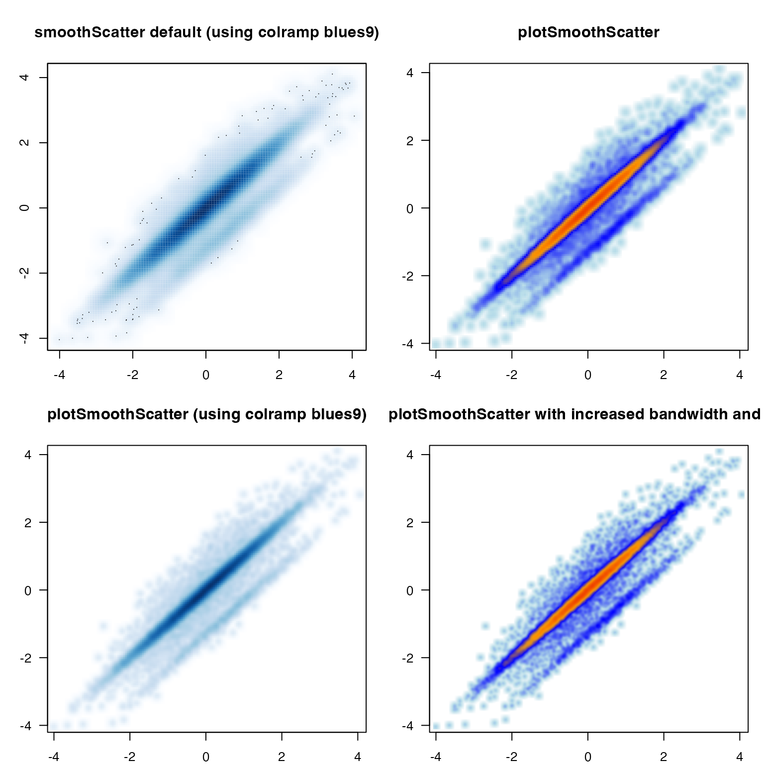

Example of smooth scatterplots using the default R function, and enhanced function in the jamba package.

`imageByColors()`

The imageByColors() function is intended to take a matrix or data.frame that already contains colors in each cell. It optionally displays cell labels when supplied.

Cell labels are grouped to display one unique label per repeated label, using the function breaksByVector() to group labels.

This function is particularly useful to simplify labels in a large table of repeated values, for example in experiment design.

Here, we define a simple data.frame composed of colors, then use the data.frame to label itself:

a1 <- c("red","blue")[c(1,1,2)];
b1 <- c("yellow","orange")[c(1,2,2)];
c1 <- c("purple","orange")[c(1,2,2)];
d1 <- c("purple","green")[c(1,2,2)];
df1 <- data.frame(a=a1, b=b1, c=c1, d=d1);
imageByColors(df1, cellnote=df1);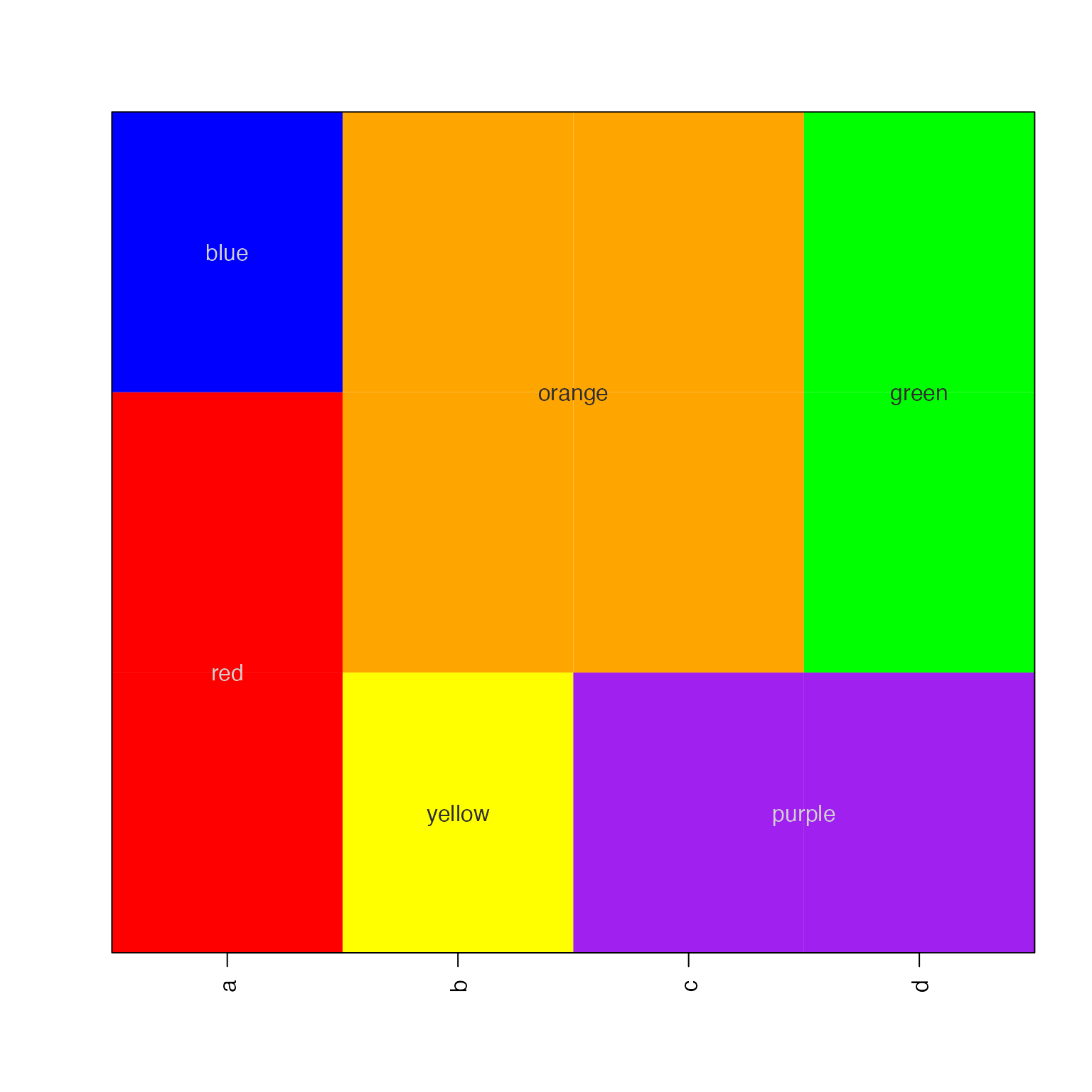

Example color matrix as plotted using the image by colors function()

Labels can be independently rotated and resized, an arbitrary example is shown below:

imageByColors(df1,
   cellnote=df1, 
   useRaster=TRUE,
   #adjBy="column",
   cexCellnote=list(c(1.5,1.5,1),
      c(1,1.5), 
      c(1.6,1.2), 
      c(1.6,1.5)),
   srtCellnote=list(c(90,0,0), 
      c(0,45), 
      c(0,0,0), 
      c(0,90,0)));

Example color matrix with rotated and grouped labels as plotted using the image by colors function.

Axis label functions

There are several useful axis labeling functions.

For log-transformed data, minorLogTicksAxis() is a flexible function to help deal with different transforms. It enables “offset”, commonly used with log2(1 + x), but now enables using any offset, e.g. log2(0.5 + x). Axis labels use integer values, accounting for the offset.

The logBase can be customized, can be properly labeled when showing log10(P-value). When showing log2 fold changes, it accepts negative values and flips the sign accordingly.

# example showing volcano plot features
set.seed(123);
n <- 1000;
vdf <- data.frame(lfc=rnorm(n) * 2)
vdf$`-log10 (padj)` <- abs(vdf$lfc) * abs(rnorm(n))
plotSmoothScatter(vdf, xaxt="n", yaxt="n", xlab="Fold change",
   main="Volcano plot\ndisplayBase=2")
logFoldAxis(1)
pvalueAxis(2)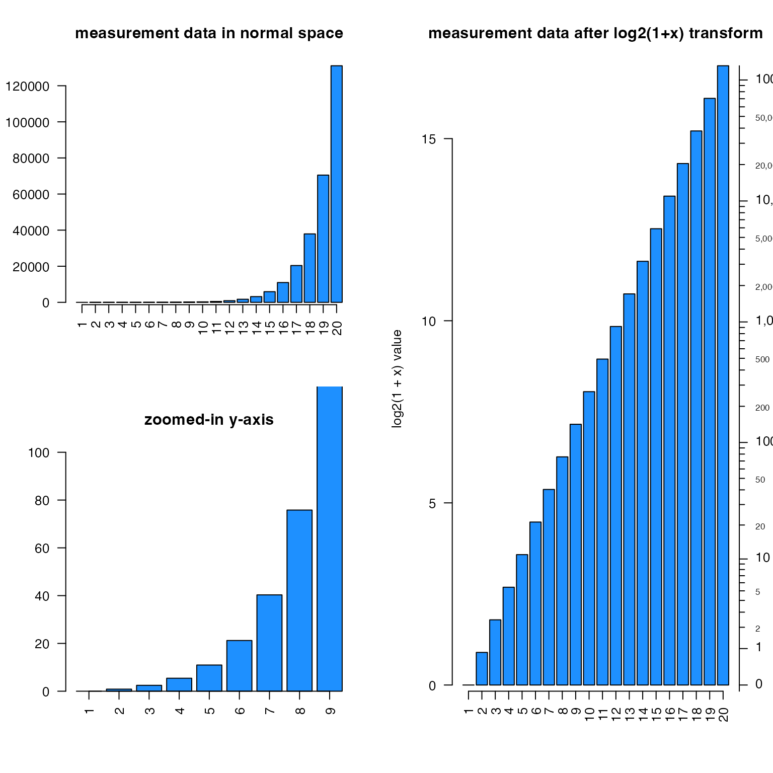

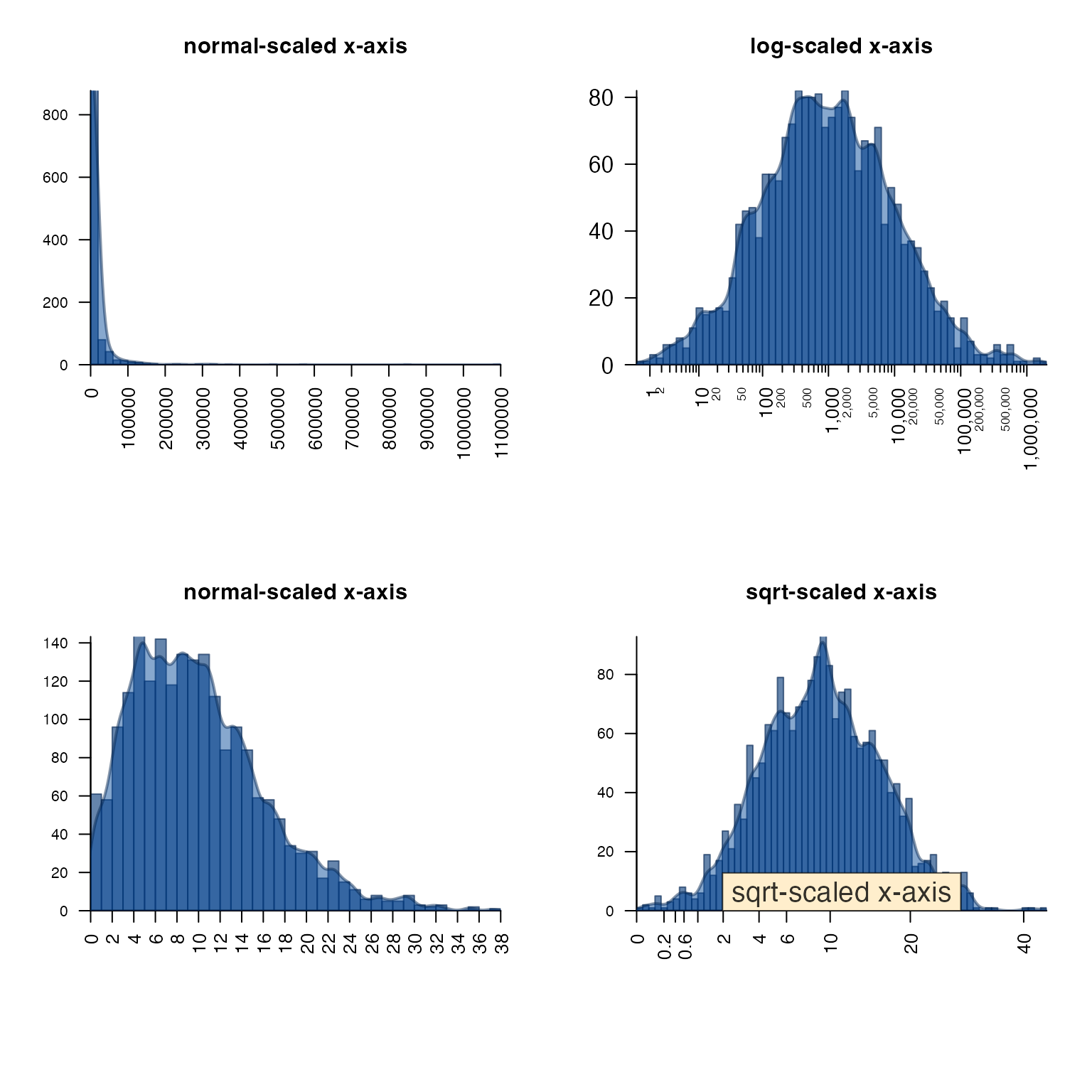
Example showing log tick axis labels with positive and negative values, and P-values.

`plotPolygonDensity()`

plotPolygonDensity() is a light wrapper around two functions: hist() and density(). However, it makes two other options convenient:

Transform the x-axis with either log10(1 + x) or sqrt(), use xScale=c("default", "log10", "sqrt").
Display multiple panels for each column of a numeric matrix.
See also: plotRidges() - a ggridges alternative.

withr::with_par(list("mar"=c(6, 4, 4, 2), "mfrow"=c(2, 2)), {
   withr::local_options(list("scipen"=7));
set.seed(123);
plotPolygonDensity(10^(3+rnorm(2000)),
   breaks=50,
   cex.axis=1,
   main="normal-scaled x-axis");
plotPolygonDensity(10^(3+rnorm(2000)),
   log="x",
   breaks=50,
   main="log-scaled x-axis");
plotPolygonDensity((3+rnorm(2000))^2,
   cex.axis=1,
   breaks=50,
   main="normal-scaled x-axis");
plotPolygonDensity((3+rnorm(2000))^2,
   cex.axis=1,
   xScale="sqrt",
   breaks=50,
   main="");
drawLabels(preset="topright",
   txt="sqrt-scaled x-axis",
   labelCex=1.5)
})

Example polygon density plot.

`drawLabels()`

drawLabels() is aimed at base R graphics, and provides a quick way to add a label to a plot. The argument preset is used to place the label relative to the sides and corners of the plot.

Shown below text_fn=jamba::shadowText will enable shadow text output.

par("mfrow"=c(1,1))
plotPolygonDensity((3+rnorm(2000))^2,
   cex.axis=1,
   xScale="sqrt",
   breaks=50,
   main="");
drawLabels(preset="bottom",
   txt="sqrt-scaled x-axis",
   text_fn=jamba::shadowText,
   labelCex=1.5)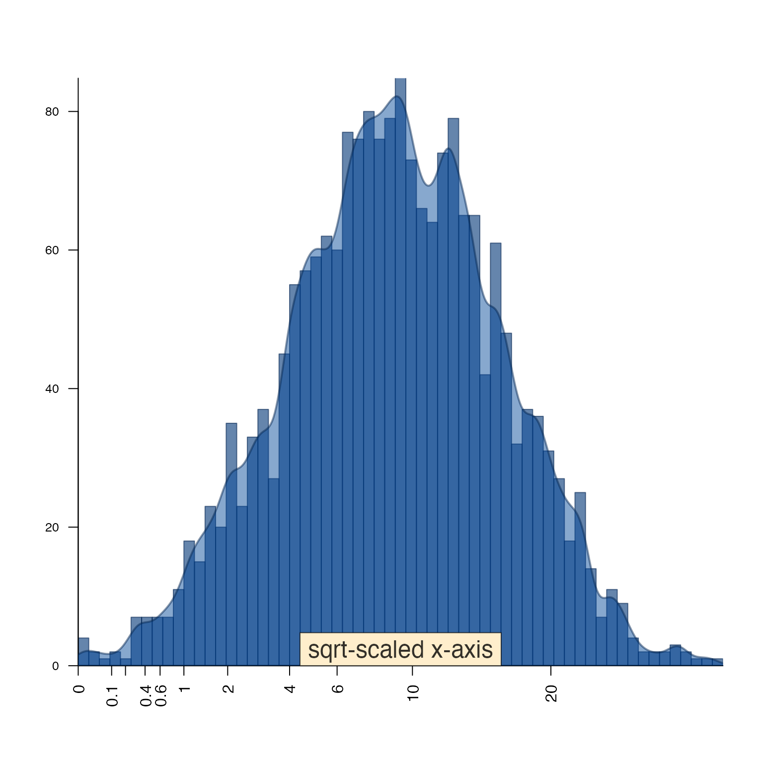

Example showing text labels, and shadow text labels on a colored background.

Colors

For me, color plays a big role in my daily work, both in how I use R, and the figures and visualizations I produce during data analysis.

Another Jam package colorjam focuses on defining categorical colors in an extensible manner.

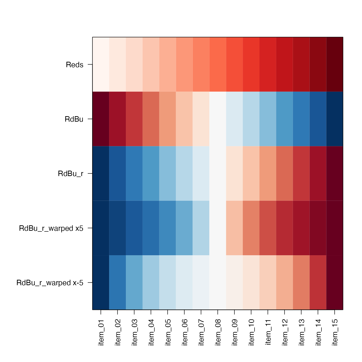
`getColorRamp()`

getColorRamp() is a workhorse of several other functions and workflows.
- It makes convenient the job of obtaining a color ramp (aka a color palette, or color gradient). It interfaces with RColorBrewer and viridisLite for color palette names, and allows some useful extensions.
- It accepts suffix "_r" to reverse color order, RColorBrewer palette "RdBu" is reversed with "RdBu_r". Red should be the high color in a heatmap - “heat”, so “RdBu_r” is recommended.

`printDebug()`

printDebug() is present in every Jam function, used when verbose=TRUE to follow the processing steps. Of course it uses color.
printDebugHtml() is used for RMarkdown output, use the chunk option results='asis' so the HTML is displayed properly.
printDebugI() is an alternative that “inverts” the color, using the color as background, with contrasting text color on top.
When a vector is provided, its values are delimited with sep, and each value is “dithered” with the same color with lighter/darker pattern for visual distinction.
Each element is assigned a color recycled from fgText, and can be customized.

printDebugHtml("printDebugHtml(): ",
  "Output is colorized: ",
  head(LETTERS, 8))

(14:38:41) 22Mar2025: printDebugHtml(): Output is colorized: A,B,C,D,E,F,G,H


withr::with_options(list(jam.htmlOut=TRUE, jam.comment=FALSE), {
  printDebugHtml(c("printDebug() using withr::with_options(): "),
    c("Output should be colorized: "),
    head(LETTERS, 8));
})

(14:38:42) 22Mar2025: printDebug() using withr::with_options(): Output should be colorized: A,B,C,D,E,F,G,H

`showColors()`

showColors() displays a color ramp, or list of color ramps, or a function as defined by circlize::colorRamp2(). (Amazing function by the way.)

Other color functions

warpRamp() is used with argument lens in other functions, and can warp the colors for more contrast. It even handles divergent colors, keeping the middle color intact.
rainbow2() is a very simple drop-in replacement for rainbow(), which adds alternating contrast to adjacent colors. A better option is colorjam::rainbowJam() but rainbow2() is a simple option until colorjam is on CRAN.

showColors(list(
   Reds=getColorRamp("Reds"),
   RdBu=getColorRamp("RdBu"),
   RdBu_r=getColorRamp("RdBu_r"),
   `RdBu_r, lens=5`=warpRamp(getColorRamp("RdBu_r"), lens=5),
   `RdBu_r, lens=-5`=warpRamp(getColorRamp("RdBu_r"), lens=-5),
   `rainbow2(15)`=rainbow2(15)
   ));

Example of color gradients using the Brewer package.

Console functions

`setPrompt()`

setPrompt() is a convenience function for R console and RStudio work, it creates a colorized R prompt with useful info: * project name * R version * Process ID (PID). The PID is useful in case ahem the R session runs wild.

Ultimately, it helps answer the question “What am I working on?”

setPrompt("jambaVignette");
# {jambaVignette}-R-3.6.0_10789>

setPrompt example

`jargs()`

Jam args().

Aligns arguments, one per row
Allows pattern search
Optionally sorts by argument name
Colorized in the R console

# all args
jargs(plotSmoothScatter)
#>                 x = ,
#>                 y = NULL,
#>              bwpi = 50,
#>             binpi = 50,
#>        bandwidthN = NULL,
#>              nbin = NULL,
#>            expand = c(0.04, 0.04),
#>       transFactor = 0.25,
#>    transformation = function( x ) x^transFactor,
#>              xlim = NULL,
#>              ylim = NULL,
#>              xlab = NULL,
#>              ylab = NULL,
#>          nrpoints = 0,
#>           colramp = c("white", "lightblue", "blue", "orange", "orangered2"),
#>               col = "black",
#>            doTest = FALSE,
#>    fillBackground = TRUE,
#>          naAction = c("remove", "floor0", "floor1"),
#>              xaxt = "s",
#>              yaxt = "s",
#>               add = FALSE,
#>               asp = NULL,
#> applyRangeCeiling = TRUE,
#>         useRaster = TRUE,
#>           verbose = FALSE,
#>               ... = 

# args with "y" in the name
jargs(plotSmoothScatter, "^y")
#>    y = NULL,
#> ylim = NULL,
#> ylab = NULL,
#> yaxt = "s"

`sdim()` and `ssdim()`

These functions apply dim() to a list, or list of lists. They recognize other S4 object types, and special types like igraph and Bioconductor objects.

It returns either data.frame of dimensions, or list of data.frame, which can be easily parsed and reviewed.

L <- list(LETTERS=LETTERS,
   letters=letters,
   lettersDF=data.frame(LETTERS, letters));
sdim(L);
#>           rows cols      class
#> LETTERS     26       character
#> letters     26       character
#> lettersDF   26    2 data.frame

L2 <- list(List1=L,
   List2=L);

sdim(L2);
#>       rows class
#> List1    3  list
#> List2    3  list
ssdim(L2)
#> $List1
#>           rows cols      class
#> LETTERS     26       character
#> letters     26       character
#> lettersDF   26    2 data.frame
#> 
#> $List2
#>           rows cols      class
#> LETTERS     26       character
#> letters     26       character
#> lettersDF   26    2 data.frame

Excel functions

`writeOpenxlsx()`

writeOpenxlsx() is a convenient wrapper for the amazing openxlsx, to automate numeric formatting, column color, font size, text alignment. When saving to Excel, you want all the details to look pretty, and to be usable without having to configure it later.

It has presets for certain data types, with default numeric formatting, and conditional color-coding by default: * P-values * fold change, log fold change * numeric values * integer values * highlight columns (bold font)

It configures some defaults: * column headers have filtering enabled * striped column and header colors * freeze pane and row to keep the header visible * column widths * word wrap, or not * header row height * categorical colors when defined

Some nice extras: * save one or more worksheets to the same file * optionally include rownames

`readOpenxlsx()`

readOpenxlsx() is convenient for reading all worksheets in an Excel file, and returns data without mangling the column headers. It returns a list of data.frame objects.

Convenience

`vigrep()`, `provigrep()`, `igrep()`, `igrepHas()`

Quick custom base::grep() for case-insensitive, or value-returning work.

vigrep() - extends grep to use value=TRUE and ignore.case=TRUE
igrep() - extends grep to use ignore.case=TRUE, case-insensitive matching.
provigrep() - progressive pattern matching, returning entries in the order they match a vector of patterns. Super useful.
igrepHas() - extends igrep() to return TRUE or FALSE, convenient for if() statements.

`gsubOrdered()`

gsubOrdered() is an extension to gsub() that preserves factor order of the input data, creating new ordered factor levels using the same gsub() replacement. Much more useful than you might think!

`pasteByRow()` and `pasteByRowOrdered()`

pasteByRow() is a lightweight by efficient method for combining multiple columns into one character string. There are other approaches, however this function is among the fastest, especially 10000 rows or more, and allows “ignoring” empty cells in the output, and trimming leading/trailing blanks.

pasteByRowOrdered() is an extension of pasteByRow() that also maintains factor level order of each column. Again, super useful to make labels that honor factor level order, for example with experimental designs.

a1 <- factor(c("mutant", "control")[c(1,1,2)],
   levels=c("control", "mutant"));
b1 <- factor(c("vehicle", "treated")[c(2,1,1)],
   levels=c("vehicle", "treated"));
d1 <- c("purple","green")[c(1,2,2)];
df2 <- data.frame(a=a1, b=b1, d=d1);
df2;
#>         a       b      d
#> 1  mutant treated purple
#> 2  mutant vehicle  green
#> 3 control vehicle  green
pasteByRow(df2);
#>                       1                       2                       3 
#> "mutant_treated_purple"  "mutant_vehicle_green" "control_vehicle_green"
pasteByRowOrdered(df2);
#>                     1                     2                     3 
#> mutant_treated_purple  mutant_vehicle_green control_vehicle_green 
#> Levels: control_vehicle_green mutant_vehicle_green mutant_treated_purple

df3 <- data.frame(df2,
   pasteByRowOrdered=pasteByRowOrdered(df2));
mixedSortDF(df3, byCols="pasteByRowOrdered")
#>         a       b      d     pasteByRowOrdered
#> 3 control vehicle  green control_vehicle_green
#> 2  mutant vehicle  green  mutant_vehicle_green
#> 1  mutant treated purple mutant_treated_purple

`makeNames()`, `nameVector()`, `nameVectorN()`

Create unique names with controlled versioning options. The base::make.unique() is great, but sometimes you need to control the output.

makeNames() returns unique names, by default for duplicated values it uses the suffix style _v1, _v2, _v3. The suffix can be controlled, whether to add a suffix to singlet entries, what number to start with, etc.
nameVector() is similar to setNames() except that it secretly runs makeNames(), and when only provided with a vector, the vector is used to define names. Named vectors are convenient with lapply() type list functions, because names are used in the returned list.

nameVectorN() creates a named vector of the vector names, useful with lapply() when you need to know the element name in the function call.

x <- rep(head(letters, 4), c(2,4,1,5));
x;
#>  [1] "a" "a" "b" "b" "b" "b" "c" "d" "d" "d" "d" "d"

makeNames(x);
#>  [1] "a_v1" "a_v2" "b_v1" "b_v2" "b_v3" "b_v4" "c"    "d_v1" "d_v2" "d_v3"
#> [11] "d_v4" "d_v5"

nameVector(x);
#> a_v1 a_v2 b_v1 b_v2 b_v3 b_v4    c d_v1 d_v2 d_v3 d_v4 d_v5 
#>  "a"  "a"  "b"  "b"  "b"  "b"  "c"  "d"  "d"  "d"  "d"  "d"

y <- nameVector(x);
nameVectorN(y);
#>   a_v1   a_v2   b_v1   b_v2   b_v3   b_v4      c   d_v1   d_v2   d_v3   d_v4 
#> "a_v1" "a_v2" "b_v1" "b_v2" "b_v3" "b_v4"    "c" "d_v1" "d_v2" "d_v3" "d_v4" 
#>   d_v5 
#> "d_v5"

lapply(nameVectorN(head(y)), function(i){
   i
})
#> $a_v1
#> [1] "a_v1"
#> 
#> $a_v2
#> [1] "a_v2"
#> 
#> $b_v1
#> [1] "b_v1"
#> 
#> $b_v2
#> [1] "b_v2"
#> 
#> $b_v3
#> [1] "b_v3"
#> 
#> $b_v4
#> [1] "b_v4"

`cPaste()`, `cPasteSU()`, `cPasteU()`

cPaste() “concatenate-paste”, takes a list and combines each vectors using a delimiter. It is among the fastest methods (at the time), partly by using S4Vectors::unstrsplit() if available. (Kudos Herve Pages!)

cPasteU() calls unique() for each vector (vectorized).
cPasteS() applies mixedSort() to each vector (vectorized).
cPasteSU() spplies sort and unique.

These functions are very useful when operating on a list of gene symbols. For example, a vector of 500,000 assay probe names may be converted to a list of gene symbols, with some assay probe names associated with multiple gene symbols. The function cPasteSU() combines gene symbols with delimiter ",", after sorting and making values unique.

It is also useful with gene-pathway data, where biological pathways are associated with a long list of gene symbols.

set.seed(123);
x <- lapply(seq_len(6), function(i){
   paste0("Gene", 
      sample(LETTERS,
         sample(c(1,1,2,5,9), 1),
         replace=TRUE));
});
cPaste(x);
#> [1] "GeneN,GeneC" "GeneR"       "GeneE,GeneT" "GeneZ"       "GeneE,GeneS"
#> [6] "GeneY,GeneY"
cPasteU(x);
#> [1] "GeneN,GeneC" "GeneR"       "GeneE,GeneT" "GeneZ"       "GeneE,GeneS"
#> [6] "GeneY"
cPasteSU(x);
#> [1] "GeneC,GeneN" "GeneR"       "GeneE,GeneT" "GeneZ"       "GeneE,GeneS"
#> [6] "GeneY"

data.frame(cPaste=cPaste(x),
   cPasteU=cPasteU(x),
   cPasteSU=cPasteSU(x))
#>        cPaste     cPasteU    cPasteSU
#> 1 GeneN,GeneC GeneN,GeneC GeneC,GeneN
#> 2       GeneR       GeneR       GeneR
#> 3 GeneE,GeneT GeneE,GeneT GeneE,GeneT
#> 4       GeneZ       GeneZ       GeneZ
#> 5 GeneE,GeneS GeneE,GeneS GeneE,GeneS
#> 6 GeneY,GeneY       GeneY       GeneY

RMarkdown Colored Tables

`kable_coloring()`

kable_coloring() - applies categorical colors to kable() output using kableExtra::kable(). It also applies a contrasting text color.

expt_df <- data.frame(
  Sample_ID="",
  Treatment=rep(c("Vehicle", "Dex"), each=6),
  Genotype=rep(c("Wildtype", "Knockout"), each=3),
  Rep=paste0("rep", c(1:3)))
expt_df$Sample_ID <- pasteByRow(expt_df[, 2:4])

# define colors
colorSub <- c(Vehicle="palegoldenrod",
  Dex="navy",
  Wildtype="gold",
  Knockout="firebrick",
  nameVector(color2gradient("grey48", n=3, dex=10), rep("rep", 3), suffix=""),
  nameVector(
    color2gradient(n=3,
      c("goldenrod1", "indianred3", "royalblue3", "darkorchid4")),
    expt_df$Sample_ID))
if (requireNamespace("kableExtra", quietly=FALSE)) {
   kbl <- kable_coloring(
     expt_df,
     caption="Experiment design table showing categorical color assignment.",
     colorSub)
}

Jamba Overview

James M. Ward

2025-03-22

Jamba Overview

Efficient alphanumeric sort

Plot functions

`plotSmoothScatter()`

`imageByColors()`

Axis label functions

`plotPolygonDensity()`

`drawLabels()`

Colors

`getColorRamp()`

`printDebug()`

`showColors()`

Other color functions

Console functions

`setPrompt()`

`jargs()`

`sdim()` and `ssdim()`

Excel functions

`writeOpenxlsx()`

`readOpenxlsx()`

Convenience

`vigrep()`, `provigrep()`, `igrep()`, `igrepHas()`

`gsubOrdered()`

`pasteByRow()` and `pasteByRowOrdered()`

`makeNames()`, `nameVector()`, `nameVectorN()`

`cPaste()`, `cPasteSU()`, `cPasteU()`

RMarkdown Colored Tables

`kable_coloring()`

Jamba Overview

James M. Ward

2025-03-22

Jamba Overview

Efficient alphanumeric sort

Plot functions

plotSmoothScatter()

imageByColors()

Axis label functions

plotPolygonDensity()

drawLabels()

Colors

getColorRamp()

printDebug()

showColors()

Other color functions

Console functions

setPrompt()

jargs()

sdim() and ssdim()

Excel functions

writeOpenxlsx()

readOpenxlsx()

Convenience

vigrep(), provigrep(), igrep(), igrepHas()

gsubOrdered()

pasteByRow() and pasteByRowOrdered()

makeNames(), nameVector(), nameVectorN()

cPaste(), cPasteSU(), cPasteU()

RMarkdown Colored Tables

kable_coloring()

`plotSmoothScatter()`

`imageByColors()`

`plotPolygonDensity()`

`drawLabels()`

`getColorRamp()`

`printDebug()`

`showColors()`

`setPrompt()`

`jargs()`

`sdim()` and `ssdim()`

`writeOpenxlsx()`

`readOpenxlsx()`

`vigrep()`, `provigrep()`, `igrep()`, `igrepHas()`

`gsubOrdered()`

`pasteByRow()` and `pasteByRowOrdered()`

`makeNames()`, `nameVector()`, `nameVectorN()`

`cPaste()`, `cPasteSU()`, `cPasteU()`

`kable_coloring()`