Smooth scatter plot with enhancements

Produce scatter plot using point density instead of displaying individual data points.

plotSmoothScatter(
  x,
  y = NULL,
  bwpi = 50,
  binpi = 50,
  bandwidthN = NULL,
  nbin = NULL,
  expand = c(0.04, 0.04),
  transFactor = 0.25,
  transformation = function(x) x^transFactor,
  xlim = NULL,
  ylim = NULL,
  xlab = NULL,
  ylab = NULL,
  nrpoints = 0,
  colramp = c("white", "lightblue", "blue", "orange", "orangered2"),
  col = "black",
  doTest = FALSE,
  fillBackground = TRUE,
  naAction = c("remove", "floor0", "floor1"),
  xaxt = "s",
  yaxt = "s",
  add = FALSE,
  asp = NULL,
  applyRangeCeiling = TRUE,
  useRaster = TRUE,
  verbose = FALSE,
  ...
)

Arguments

x

numeric vector, or data matrix with two or more columns.

y

numeric vector, or if data is supplied via x as a matrix, y is NULL.

bwpi

numeric value indicating the bandwidth "per inch" to scale the bandwidth based upon visual space available. This argument is used to define bandwidthN, however bwpi is only used when bandwidthN=NULL. The bandwidth is used to define the 2-dimensional point density.

binpi

numeric value indicating the number of bins "per inch", to scale based upon visual space available. This argument is used to define nbin, however binpi is only used when nbin=NULL.

bandwidthN

integer number of bandwidth steps to use across the visible plot window. Note that this bandwidth differs from default graphics::smoothScatter() in that it uses the visible plot window instead of the data range, so if the plot window is not sufficiently similar to the data range, the resulting smoothed density will not be visibly distorted. This parameter also permits display of higher (or lower) level of detail.

nbin

integer number of bins to use when converting the kernel density result (which uses bandwidthN above) into a usable image. This setting is effectively the resolution of rendering the bandwidth density in terms of visible pixels. For example nbin=256 will create 256 visible pixels wide and tall in each plot panel; and nbin=32 will create 32 visible pixels, with lower detail which may be suitable for multi-panel plots. To use a variable number of bins, try binpi.

expand

numeric value indicating the fraction of the x-axis and y-axis ranges to add to create an expanded range, used when add=FALSE. The default expand=c(0.04, 0.04) mimics the R base plot default which adds 4 percent total, therefore 2 percent to each side of the visible range.

transFactor

numeric value used by the default transformation function, which effectively scales the density of points to a reasonable visible distribution. This argument is a convenience method to avoid having to type out the full transformation function.

transformation

function which converts point density to a number, typically related to square root or cube root transformation. Note that the default uses transFactor but if a custom function is supplied, it will not use transFactor unless specified.

xlim

numeric x-axis range, or NULL to use the data range.

ylim

numeric y-axis range, or NULL to use the data range.

xlab, ylab

character labels for x- and y-axis, respectively.

nrpoints

integer number of outlier datapoints to display, as defined by graphics::smoothScatter(), however the default here is nrpoints=0 to avoid additional clutter in the output, and because the default arguments bwpi, binpi usually indicate all individual points.

colramp

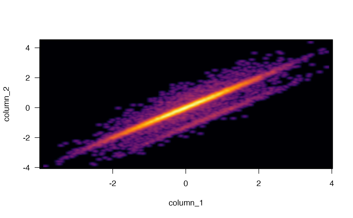
any input recognized by getColorRamp():

• character vector with multiple colors

• character string length 1, with valid R color used to create a linear color gradient

• character name of a known color gradient from RColorBrewer or viridis

• function that itself produces vector of colors, in the form function(n) where n defines the number of colors.

col

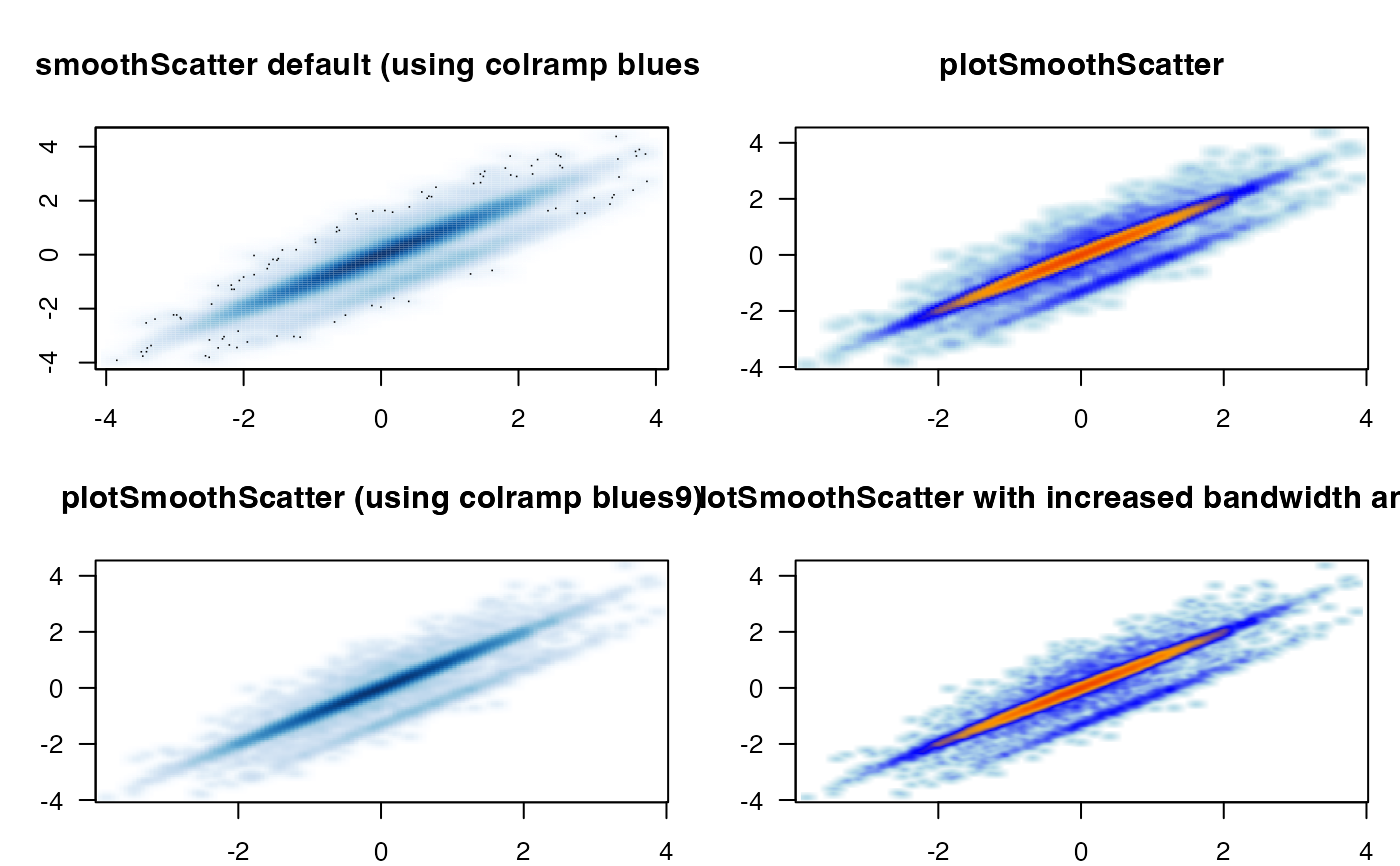
character string with R color used when nrpoints is non-zero, this color defines the color of those points.

doTest

logical indicating whether to create a visual set of test plots to demonstrate the utility of this function.

fillBackground

logical indicating whether to fill the background of the plot panel with the first color in colramp. The default fillBackground=TRUE is useful since the plot panel may be slightly wider than the range of data being displayed, and when the first color in colramp is not the same as the plot device background color. Run a test using: plotSmoothScatter(doTest=TRUE, fillBackground=FALSE, colramp="viridis") and compare with: plotSmoothScatter(doTest=TRUE, colramp="viridis")

naAction

character string indicating how to handle NA values, typically when x is NA and y is not NA, or vice versa. valid values:

"remove"

ignore any points where either x or y are NA

"floor0"

change any NA values to zero 0 for either x or y

"floor1"

change any NA values to one 1 for either x or y

The latter two options are useful when the desired plot should indicate the presence of an NA value in either x or y, while also indicating the the corresponding non-NA value in the opposing axis. The driving use was plotting gene fold changes from two experiments, where the two experiments may not have measured the same genes.

xaxt

character value compatible with par(xaxt), used to control the x-axis range, similar to its use in plot() generic functions.

yaxt

character value compatible with par(yaxt), used to control the y-axis range, similar to its use in plot() generic functions.

add

logical whether to add to an existing active R plot, or create a new plot window.

asp

numeric with optional aspect ratio, as described in graphics::plot.window(), where asp=1 defines x- and y-axis coordinate ranges such that distances between points are rendered accurately. One data unit on the y-axis is equal in length to asp multiplied by one data unit on the x-axis. Notes:

• When add=TRUE, the value asp is ignored, because the existing plot device is re-used.

• When add=FALSE and asp is defined with numeric value, a new plot device is opened using plot.window(), and the xlim and ylim values are passed to that function. As a result the par("usr") values are used to define xlim and ylim for the purpose of determining visible points, relevant to applyRangeCeiling.

applyRangeCeiling

logical indicating how to handle points outside the visible plot range. Valid values:

TRUE

Points outside the viewing area are fixed to the plot boundaries, in order to represent that there are additional points outside the boundary. This setting is recommended when the reasonable viewing area is smaller than the actual data, for example to be consistent across plot panels, but where you want to indicate that points may be outside the range.

FALSE

Points outside the viewing area is not displayed, with no special visual indication. This setting is useful when data may contain a large number of points at c(0, 0) and the density overwhelms the detail in the rest of the plot. In that case setting xlim=c(1e-10, 10) and applyRangeCeiling=FALSE would obscure these points.

useRaster

logical indicating whether to produce plots using the graphics::rasterImage() function which produces a plot raster image offline then scales this image to visible plot space. This technique has two benefits:

1. It produces substantially faster plot output.

2. Output contains substantially fewer plot objects, which results in much smaller file sizes when saving in PDF or SVG format.

verbose

logical indicating whether to print verbose output.

...

additional arguments are passed to called functions, including getColorRamp(), nullPlot(), smoothScatterJam().

Details

This function intends to make several potentially customizable features of graphics::smoothScatter() plots much easier to customize. For example bandwidthN allows defining the number of bandwidth steps used by the kernel density function, and importantly bases the number of steps on the visible plot window, and not the range of data, which can differ substantially. The nbin argument is related, but is used to define the level of detail used in the image function, which when plotting numerous smaller panels, can be useful to reduce unnecessary visual details.

This function also by default produces a raster image plot with useRaster=TRUE, which adjusts the x- and y-bandwidth to produce visually round density even when the x- and y-ranges are very different.

Comments:

• asp=1 will define an aspect ratio 1, meaning the x-axis and y-axis units will be the same physical size in the output device. When this is true, and fillBackground=TRUE the xlim and ylim values follow logic for plot.default() and plot.window() such that each axis will include at least the xlim and ylim ranges, with additional range included in order to maintain the plot aspect ratio.

• When asp, and any of xlim or ylim, are defined, the data will be "cropped" to respective xlim and ylim values as relevant, after which the plot is drawn with the appropriate plot aspect ratio. When applyRangeCeiling=TRUE, points outside the fixed xlim and ylim range are fixed to the edge of the range, after which the plot is drawn with the requested plot aspect ratio. It is recommended not to define xlim and ylim when also defining asp.

• When add=TRUE the xlim and ylim values are already defined by the plot device. It is recommended not to define xlim and ylim when add=TRUE.

See also

Other jam plot functions: adjustAxisLabelMargins(), coordPresets(), decideMfrow(), drawLabels(), getPlotAspect(), groupedAxis(), imageByColors(), imageDefault(), minorLogTicksAxis(), nullPlot(), plotPolygonDensity(), plotRidges(), shadowText_options(), shadowText(), showColors(), smoothScatterJam(), sqrtAxis(), usrBox()

Examples

# doTest=TRUE invisibly returns the test data
x <- plotSmoothScatter(doTest=TRUE);


# so it can be plotted again with different settings
colnames(x) <- c("column_1", "column_2")
plotSmoothScatter(x, colramp="inferno");