2.2 Specialized Input Types
The driving motivation for Venndir involved gene expression data, and there are several common methods to import differentially expressed genes.
2.2.1 limma
The limma (Smyth et al. 2025) package covers an amazing array of gene and Omics expression analysis methods, spanning transcript and proteomics microarray data, transcriptomics RNA sequencing (RNA-seq) data, and a broad range of other data types including proteomics, lipidomics, metabolomics, and DNA methylation.
The common paradigm, beginning with x as expression data.
See limma::getEAWP() for a description of all recognized data
object types.
library(limma)

# fit linear model
fit <- lmFit(x, design=design)

# apply contrasts
fit2 <- contrasts.fit(fit, contrasts=contrasts)

# Optional Empirical Bayes moderated t-statistic
fit3 <- eBayes(fit)
Now one would use fit3, or fit2 if eBayes was not necessary, to
summarize the statistical contrasts.
Two common approaches are used here, both can be valid:
- Extract each contrast into a
data.frameusinglimma::topTable(), then follow List of data frames. - Use
limma::decideTests()to filter all contrasts together. This function returnslimma::TestResults-classwhich is equivalent to Signed incidence matrix.
For example, to filter by adjusted P-value 0.05, and 1.5-fold change:
The resulting incidence matrix im contains one
column per contrast.
When using only a subset of contrasts, use the argument sets as
described in Consistent Set Colors.
The example below chooses sets=c(1, 3).
2.2.2 DESeq2
DESeq2 (Love, Anders, and Huber 2025) is widely used and excellent for RNA-seq analysis.
The example below is adapted from DESeq2::DESeq() to use three groups:
'A', 'B', 'C'.
The following code sets up some test data.
suppressPackageStartupMessages(library(DESeq2))
set.seed(123)
cnts <- matrix(rnbinom(n=1500, mu=100, size=1/0.5), ncol=15)
rownames(cnts) <- paste0("row", jamba::padInteger(1:100))
cond <- factor(rep(LETTERS[1:3], each=5))
colnames(cnts) <- jamba::makeNames(cond, suffix="")
cnts[1, 1:5 + 0] <- cnts[1, 1:5] + 275;
cnts[2, 1:5 + 5] <- cnts[2, 1:5 + 5] + 355;
cnts[3, 1:5 + 10] <- cnts[3, 1:5 + 10] + 425;
cnts[4, 1:5 + 10] <- cnts[4, 1:5 + 10] + 655;

# object construction
suppressMessages(
   dds <- DESeqDataSetFromMatrix(cnts, DataFrame(cond), ~ cond)
)

# standard analysis
suppressMessages(
   dds <- DESeq(dds)
)
The object dds can be used to extract statistical results
for each contrast, for example see DESeq2::resultsNames(dds).
The next steps extract a DESeqResults object for each contrast
of interest. Note: Use whichever method you typically use at
this point, there are too many possible workflows to cover here.
# Contrast: 'B - A'
resBA <- results(dds, contrast=c("cond", "B", "A"))

# Contrast: 'C - A'
resCA <- results(dds, contrast=c("cond", "C", "A"))

# Print the first few rows of the "C - A" contrast results
head(data.frame(check.names=FALSE, resCA))
(fig:deseq2-example2-real) The first 6 rows following DESeq2 statistical analysis.
| baseMean | log2FoldChange | lfcSE | stat | pvalue | padj | |
|---|---|---|---|---|---|---|
| row001 | 176.5 | -1.48 | 0.63 | -2.36 | 0.0181392 | 0.3023208 |
| row002 | 188.8 | -0.24 | 0.65 | -0.37 | 0.7096112 | 0.9355705 |
| row003 | 262.0 | 1.85 | 0.45 | 4.08 | 0.0000453 | 0.0022649 |
| row004 | 294.1 | 3.11 | 0.59 | 5.30 | 0.0000001 | 0.0000118 |
| row005 | 82.5 | -0.47 | 0.50 | -0.93 | 0.3502942 | 0.7961232 |
| row006 | 87.5 | -0.16 | 0.67 | -0.24 | 0.8121139 | 0.9443185 |
Two steps are applied, intentionally lenient for this example:
- Filter by statistical thresholds
- adjusted P-value
padj < 0.20 - fold change
abs(log2FoldChange) > log2(1)
- adjusted P-value
- Convert to signed set, assigning names using the DESeq2 result rownames.
# filter statistics
resBA_hitdf <- subset(resBA,
   padj <= 0.2 &
   abs(log2FoldChange) > log2(1))

# generate named vector
resBA_hits <- setNames(
   sign(resBA_hitdf$log2FoldChange),
   rownames(resBA_hitdf))

resBA_hits
## row001 row002 row022 row023 row040 row045 row096
## -1 1 1 1 -1 1 1The same steps are performed for contrast 'C - A'.
resCA_hitdf <- subset(resCA,
   padj <= 0.2 &
   abs(log2FoldChange) > log2(1))
resCA_hits <- setNames(
   sign(resCA_hitdf$log2FoldChange),
   rownames(resCA_hitdf))

resCA_hits
## row003 row004 row023 row045 row056
## 1 1 1 1 1The two signed sets are combined into a list then
visualized with venndir() in Figure 2.12.
setlist <- list(
   "B-A"=resBA_hits,
   "C-A"=resCA_hits)
v <- venndir(setlist,
   legend_headers=c(Set="Contrast", Size="Differential Genes"))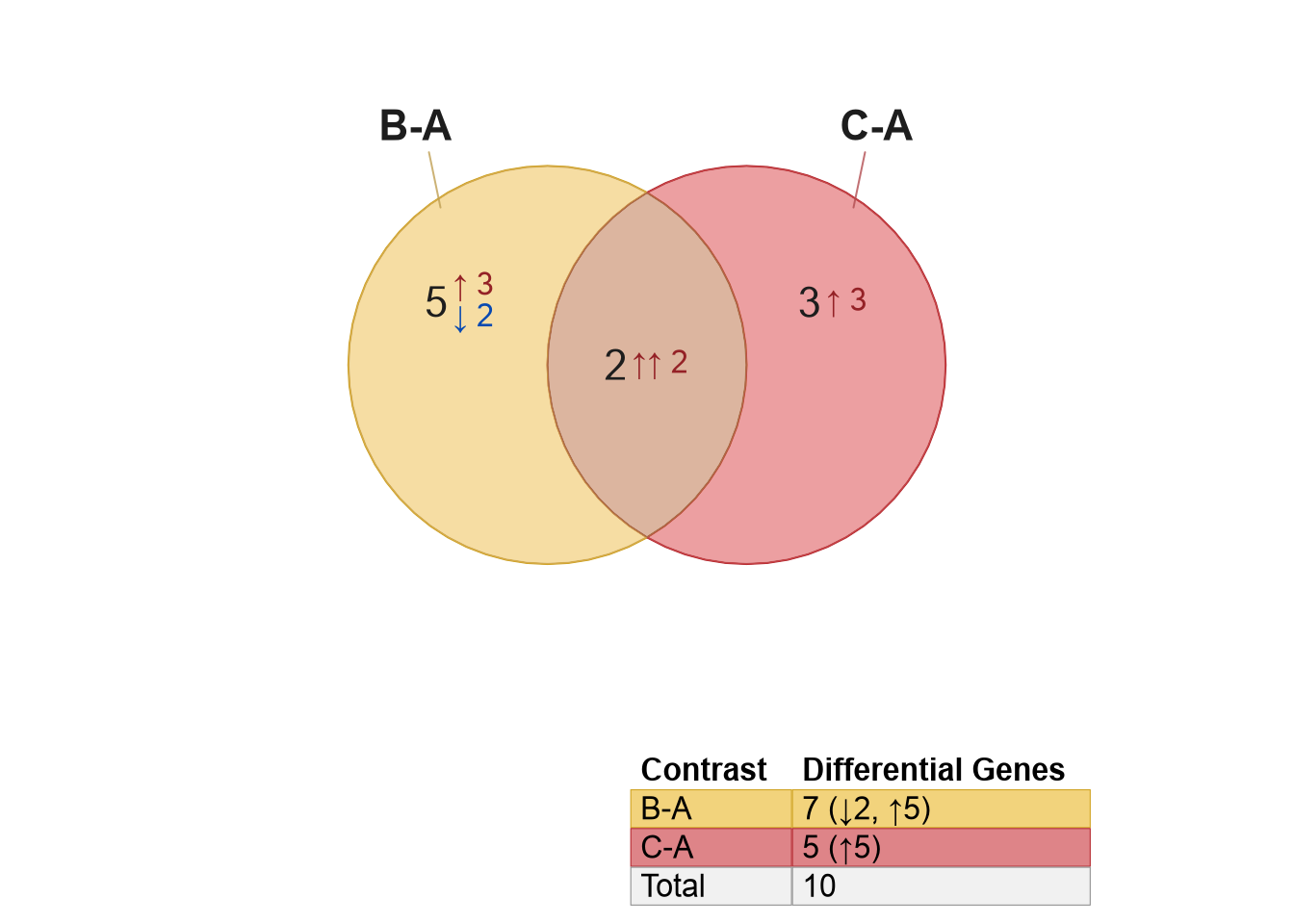
Figure 2.12: Directional Venn diagram comparing statistical hits from two contrasts analyzed using DESeq2.
To view the genes in the Venn diagram, skip ahead to Item labels and
Signed items, or to extract the genes use overlaplist(v).