4.13 Venndir Graphics Objects
The Venndir object also stores the grid graphical objects (grobs)
used for visualization, however the grobs are only created by calling
plot() or render_venndir(). The output of this function is Venndir
object with hidden attributes which contain grobs.
When calling venndir(), two options may be useful:
do_plot=TRUE: This argument causesvenndir()to callrender_venndir(), which then creates the relevant grobs.do_draw=FALSE: This argument is passed torender_venndir(), so the grobs are not drawn to the graphical device.
The following example creates a Venndir object without creating
a new plot, and which creates all the necessary grobs.
v <- venndir(make_venn_test(),
   show_labels="Ni",
   main="Plot Title",
   fontfamily="Arial",
   do_plot=TRUE,
   do_draw=FALSE,
   poly_alpha=0.4,
   item_cex_factor=0.6,
   legend_color_style=c("black", "blackborder"))
The relevant attribute names are described as follows:
'gtree': the singlegridobject that contains all Venndir grobs.'grob_list': thelistof eachgridobject, separated by type.'viewport': thegridobject representing the graphicsviewport.'adjx',adjy': the adjustment function used to convertJamPolygoncoordinates to unit 'nspc' scaled values between 0 and 1.
4.13.1 Venndir gtree
The 'gtree' attribute contains a grid:gTree object, which can be
drawn directly. The gtree object already contains the relevant
viewport.
Figure 4.23 shows the plot after drawing the 'gtree' attribute.
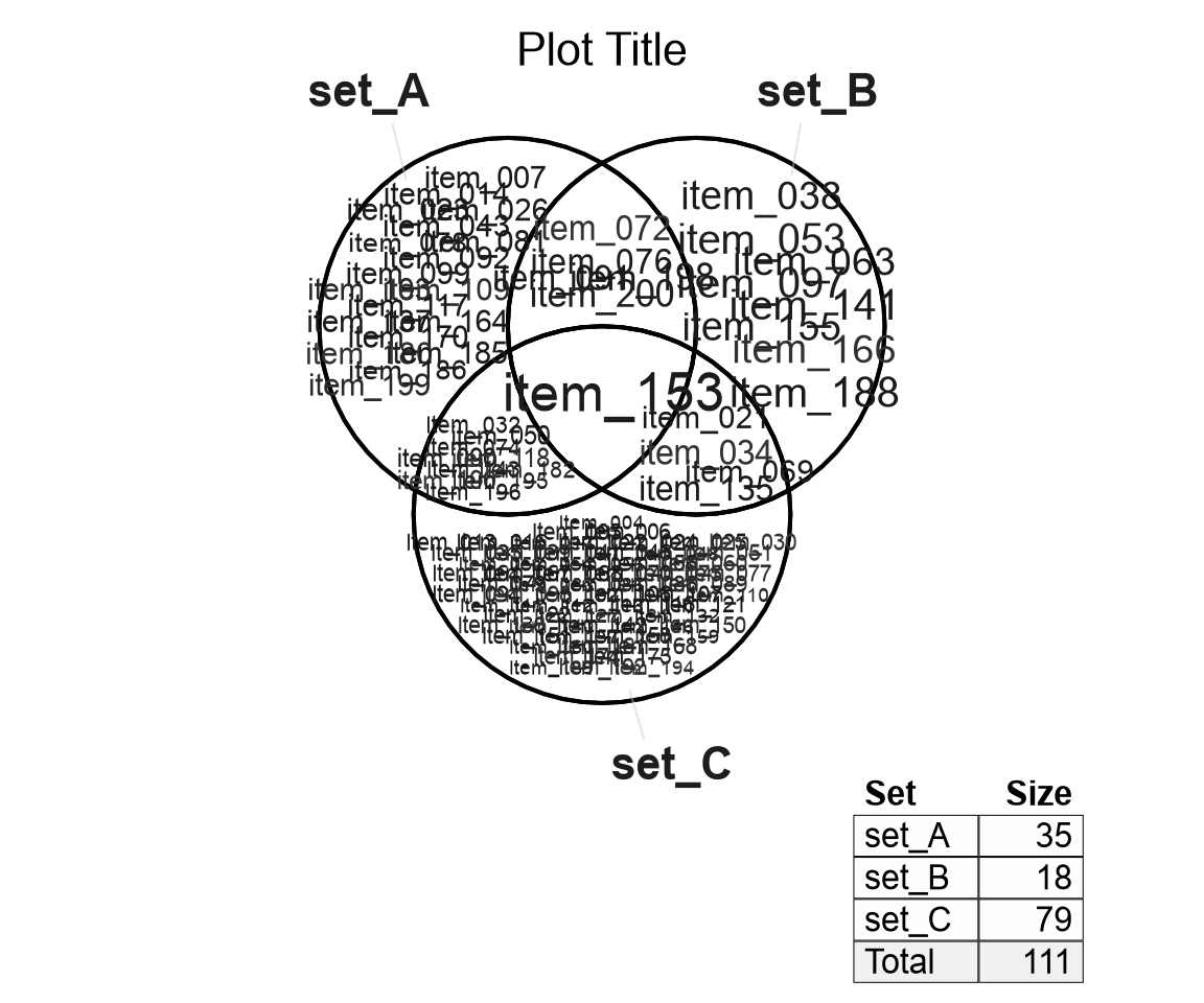
Figure 4.23: Venn diagram created by drawing the 'gtree' attribute object.
A detailed list of all grobs within the gtree can be seen by calling
grid::grid.ls(), however it is not listed here because it contains
over 350 grobs!
4.13.2 Venndir grob_list
An alternative representation is the 'grob_list' attribute,
which is a list with each Venndir visual component. The exact
elements may vary dependent upon which options were used.
The purpose of inspecting grid grobs is mainly to allow direct
manipulation of the grobs, for advanced customizations for example.
Each individual component can be edited in detail.
The grobs by type are described below:
'jps': theJamPolygonobject with polygons and border.'item_labels': item labels, only if enabled by argumentshow_labels.'labels': themarqueegrobs used for all text labels.'segments': the line segments connecting labels to polygons, where relevant.'legend': thegridobject representing the Venndir legend, if relevant.'main_title': the title object, only if defined by argumentmain.
Figure 4.24 shows the plot after drawing each grid component
from the 'grob_list' attribute.
grob_list <- attr(v, "grob_list");

grid::grid.newpage()
grid::grid.draw(grob_list$jps)
grid::grid.draw(grob_list$item_labels)
grid::grid.draw(grob_list$labels)
grid::grid.draw(grob_list$segments)
grid::grid.draw(grob_list$legend)
grid::grid.draw(grob_list$main_title)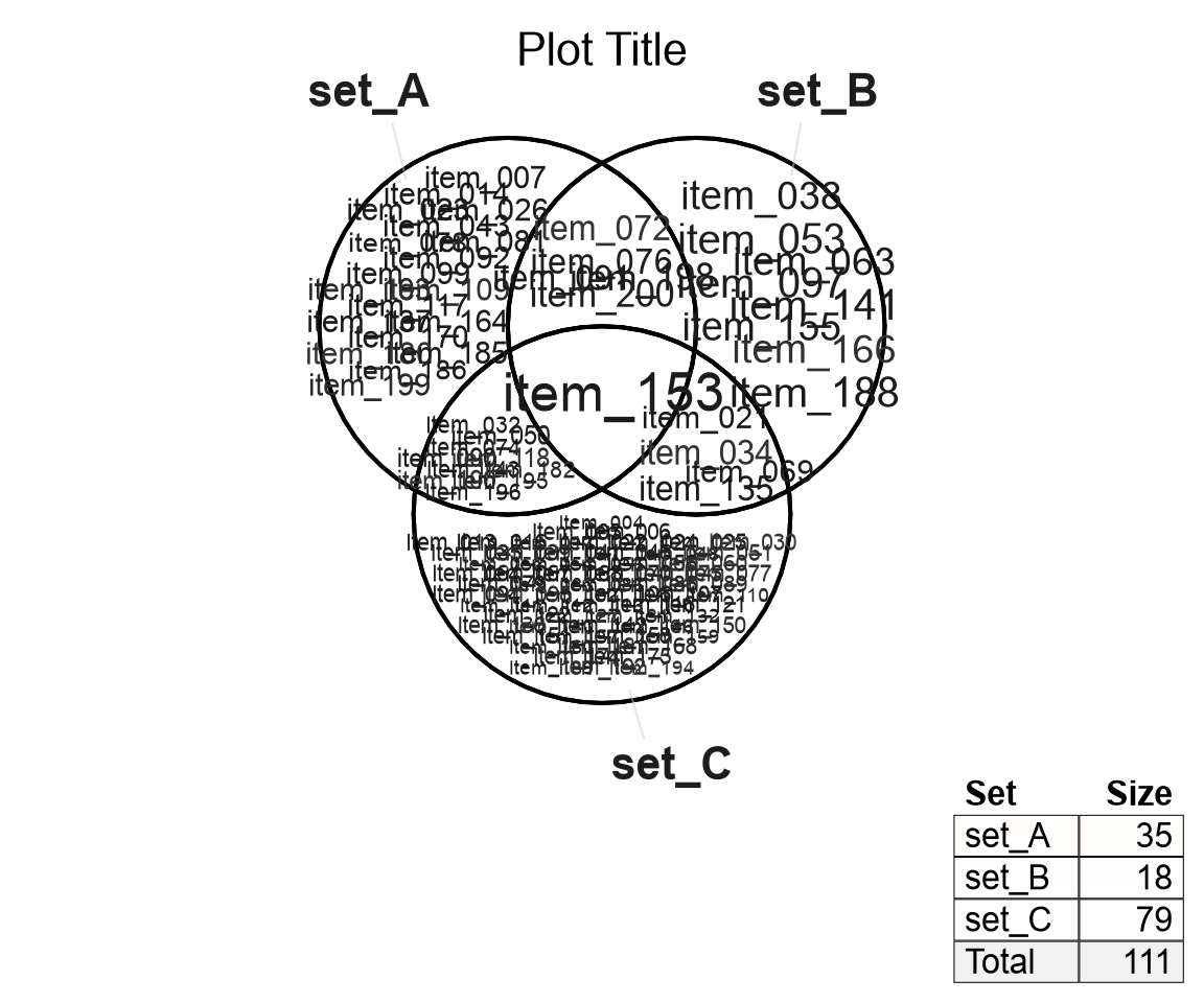
Figure 4.24: Venn diagram created by drawing each component in the 'grob_list' attribute.
4.13.3 Manipulate grob_list
The entries are named to be reognizable, for example the grob names
in the 'jps' entry are listed with grid::grid.ls():
## jps
##   set_A|set:pathGrob:outer:1
##   set_A|set:pathGrob
##   set_B|set:pathGrob:outer:1
##   set_B|set:pathGrob
##   set_C|set:pathGrob:outer:1
##   set_C|set:pathGrob
##   set_A:pathGrob:inner
##   set_A:pathGrob:inner:1
##   set_A:pathGrob
##   set_B:pathGrob:inner
##   set_B:pathGrob:inner:1
##   set_B:pathGrob
##   set_C:pathGrob:inner
##   set_C:pathGrob:inner:1
##   set_C:pathGrob
##   set_A&set_B:pathGrob:inner
##   set_A&set_B:pathGrob:inner:1
##   set_A&set_B:pathGrob
##   set_A&set_C:pathGrob:inner
##   set_A&set_C:pathGrob:inner:1
##   set_A&set_C:pathGrob
##   set_B&set_C:pathGrob:inner
##   set_B&set_C:pathGrob:inner:1
##   set_B&set_C:pathGrob
##   set_A&set_B&set_C:pathGrob:inner
##   set_A&set_B&set_C:pathGrob:inner:1
##   set_A&set_B&set_C:pathGrob
Each polygon is named with substring up to the first ':' colon, after which are optional modifiers indicating the border applied, in order:
- Each polygon is drawn with outer border (if outerborder is defined),
- then polygon fill and border (if border is defined),
- then inner fill (if innerborder is defined),
- then inner border (if innerborder is defined).
As described in Venndir Rendering Steps, a polygon is drawn for each full set, denoted with polygon names having '|set' at the end. Then each overlap region is drawn, where polygons are named by the overlap sets.
The example below is somewhat advanced, and demonstrates how to
extract a specific polygon grob, use it to create a custom pattern
fill, then reinsert the new grob into the grob_list.
First, extract one overlap region, and draw it to confirm:
grobname <- "set_C:pathGrob:inner"
use_grob <- grid::getGrob(grob_list$jps, gPath=grobname)
grid::grid.newpage();
grid::grid.draw(use_grob)
Figure 4.25: One overlap polygon is extracted from grob_list and drawn.
The next step is to define a grid pattern, in this case it requires the gridpattern R package, loading an image.
Another alternative is to define a color gradient, for example
with gridpattern::grid.pattern_gradient().
bg_file <- "images/water_bg.png"
bg_pat <- gridpattern::grid.pattern_image(filename=bg_file,
   type="tile", scale=1, draw=FALSE)
Now the grob use_grob is used to apply a clipping region to
the pattern fill, so the pattern is only applied to this
specific polygon region.
# clip background to the grob
clipped_name <- paste0(grobname, ".pattern")
clipped <- list(gridpattern::clippingPathGrob(
   clippee=bg_pat,
   clipper=use_grob,
   name=clipped_name));
names(clipped) <- clipped_name
Now draw the clipped background image:

Figure 4.26: (ref:groblist-clip-draw)
Finally, re-insert the background into the grob_list:
grob_list_jps_list <- grob_list$jps$children;
grobmatch <- match(grobname, names(grob_list_jps_list));

if (grobmatch == 1) {
   grob_list_jps_list <- append(grob_list_jps_list,
      clipped,
      after=grobmatch - 1)
} else {
   grob_list_jps_list <- append(clipped,
      grob_list_jps_list,
      after=1)
}
# insert into grob_list
grob_list$jps <- grid::grobTree(
   children=do.call(grid::gList, grob_list_jps_list),
   name="jps")
Bonus points: Re-create the grob tree gTree object:
# make new gTree
jps_gtree <- grid::grobTree(
   children=do.call(grid::gList, grob_list),
   name="venndir.figure")
Drawing the gTree is sometimes more convenient than drawing
each element in the grob_list:
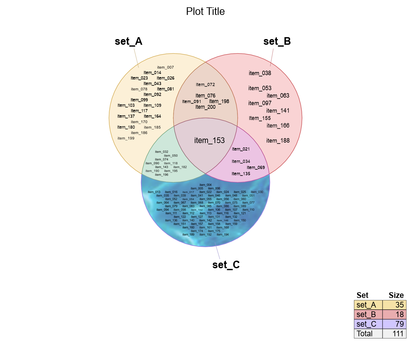
Figure 4.27: The custom Venndir figure is drawn, using pattern fill in one overlap region.
Note that the original polygon fill is drawn on top of the pattern fill, but this layer could be removed so the pattern is shown without interference. This change is left to the reader.